7 The quality of raw data
One of the most annoying aspects of data science is the time that you have to spend on repairing and reading raw data stored in inconvenient and inconsistent ways. I sometimes spend 20%-30% of the time needed to analyze a data set on understanding how it was stored, what is stored where and on repairing the data. The best illustration of the problem is given by an example.
Messy data
Please download the Excel file under the link called Download an untidy version on the Data Carpentry for Biologists website “Improving Messy Data” and open it.
Try to answer the following questions:
- do you understand what the entries -999 under
Weightmean? - do you understand what the questionmark under the
Weightcolumn means? - do you know in which year the data under
Plot: 3was gathered?
And
- which problems do you foresee when reading this data using the
read_excel()function? - will
read_excel()be able to read whether a cell was gray-colored? - how will you know in which plot the data was gathered once you managed to read the data?
Apart from the fact that data needs to have a good experimental quality, data must also be stored in a way that supports reproducible analysis, and minimizes effort and mistakes during the analysis phase. In short, data should be stored in a consistent, unambiguous and concise manner. The only way to reach this goal is to follow a number of rules when the data set is generated.
7.1 Seven rules for formating raw data
Lots of data are stored in free style text, for example in scientific articles, and in many cases it is impossible to structure such data in a way that facilitates reading by machines. However, some data can be stored in a structured manner, and that is the type we are talking about in this course, because this type of data is amenable to automated analysis. Most structured data can be stored in one table or multiple related tables. These tables contain variables and cases or observations, usually organized in columns and rows. The cells contain values, one value for each observation and variable. The following rules pertaining to the organization of data in tables will guarantee optimal and frictionles use of these data.
Rule 1: Give each variable its own column
A variable is one particular aspect of a case or observation that you measure or asses. Often, variables have a unit. To simplify working with these data it’s important to give every variable its own column; technically speaking, to store data in an atomic format. This is also called level 1 database normalization. In practice this means the following:
- Do not combine variables: for example, a researcher scores the sex of an animal specimen (M, F) but in case of uncertainty uses the values M+ and F+ to indicate that fact. Or, he scores juvenile male and female individuals as Mj and Fj. What is actually scored in both cases is a combination of two variables. In the first case it is sex (M, F) and uncertain_sex (TRUE, FALSE), and in the second it is sex (M, F) and juvenile (TRUE, FALSE). If during data analysis you want to remove the juvenile specimens or those of which the sex is uncertain, or you want to indicate them with special symbols in a graph then that can be much easier accomplished if these variables have been recorded in separate columns.
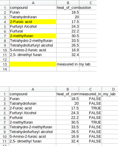
- Do not use cell formatting to convey information: this is especially relevant if you use a spreadsheet program. Cell formatting, like cell color, font color and font type are difficult or impossible to read for most analysis software. Equivalent to the previous case, actually two atomic pieces of information have been stored here. Instead of using cell formatting, you should create a new variable that conveys the information that was originally conveyed by the format:
- Put comments in a separate column: if you add a comment in a cell, like sex: “F, specimen was severely damaged”, then split this information into two columns, one called sex and another called comment. In fact, if the comment implies that the value F was not clear, the following rule applies.
- Label bad or uncertain data using a separate binary or factor variable with a name like bad_data. Such a separate variable makes it much easier to remove these observations before an analysis, or to indicate them by special symbols in a graph. Never remove bad data from the original data files!
Rule 2: Avoid using variable names with spaces or having special characters
Many programs have trouble using variable names with spaces, and even if they don’t, it’s often cumbersome to work with them. Instead of a variable name like body weight you should convert it to the camel case bodyWeight or, safer even because some programs are case-insensitive, the snake case body_weight.
Rule 3: Give every observation its own row
This means that you should avoid using column names that are actually variable values (not variable names). An example of is this is a table of weights of males and females of different bird species (Figure 7.2).

sex. This has been converted to a table with two new columns. Clearly, the original species_name column has to be repeated for every value of sex. The lower format is the preferred format for most tasks in data analysis.
- Put replicate measurements in a single column. An often encountered variant of the previous pattern is when researchers put replicate measurements in consecutive columns, with names like optical_density_1, optical_density_2, etc. An example of this is discussed in Chapter 11.

When carefully considering this case, we should conclude that these two columns either represent one variable optical_density, or two variables optical_density and replicate_nr. The latter is the case if the replicate number actually represents the order in which the replicates were measured, and is not randomly assigned. In this case the replicate number conveys information about an experimental fact. This can be important information, as the timing of replicate measurements sometimes introduces bias. You can only detect this if both pieces of information, the measurement and the replicate number, are recorded as separate variables.
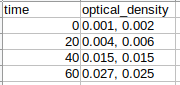
- Do not put replicate observations in one cell. This is a variant of the previous example. The following optical density column may be very hard to parse by data analysis software. You can’t use these cells in spreadsheet calculations either.
Rule 4: Split data into different tables if you would (often) repeat a combination of variables
The following example demonstrates this rule. The figure below shows the first 20 rows of a table with almost 35000 observations on animals in a desert plot.
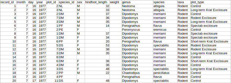
Note that the genus species and taxa repeat the same values for each species identified by the value in the column species_id. For example, Merriam’s kangaroo rat (Dipodomys merriami) is observed many times (species_id: DM; genus: Dipodomys; species: merriami; taxa: Rodent). Clearly, the combinations of these values will not change between different observations. Therefore, according to this rule, this table should be split into two tables, one with information directly related to the observation, and another with information directly related to the species. The link between both tables is provided by the unique species identifier species_id. In fact, the species table belonging to this data set contains only 48 species, a part of which is shown below.
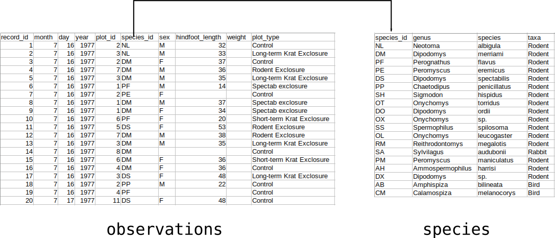
The splitting of the original table into two tables has two advantages. The first is that the total storage space of these tables is less than that of the original table, because we have removed redundant combinations in columns. The more important advantage is that we have removed a potential source of error, because every time the information about a species is entered, especially when there is any manual interference in this process, there is the risk of entering errors. Also, if we found out later that there is a mistake in a genus name, we would have to correct that in thousands of rows in the combined table, whereas we only have to correct it one row in the split tables. As a rule to determine whether and how you should split data into different tables you should ask the question whether a table contains information about obviously different entities, like here species and observations.
Are there other ways to split these tables and remove even more redundancy? How do you determine the balance between removing redundancy and creating many tables that have to be linked again afterwards?
Answer
Yes, for example by making a table called plots containingplot_id and plot_type. Possibly also by splitting the species table into species, genus and taxa tables. The latter will not remove much redundancy, given the fact that the species table contains only 48 species. So, we might decide not to split the species table to save making many tables.
Rule 5: Use consistent values
Clearly, you should not mix values M and m and F and f to score sex if M and m or F and f are supposed to mean the same thing. Other examples: mixing the use of True, T, 1 etc. when they are supposed to mean the same. Since these values are different, they will be treated as being different in software for data analysis, even though in your opinion they mean the same. A sneaky variation on this theme are the leading and trailing spaces which are usually very difficult to detect: “ M” or “M ” or “M” will be interpreted as different values!
Rule 6: Use empty positions for missing data
And be consistent in using this value. Or, if you think this is not explicit enough you could use the value NA. Some people use -999, 999, -, 0, etc. Do not use such codes, because they are easily interpreted as numbers in data analysis software, and thus lead to mistakes! See, for example, how encoding missing data as 101 led to a serious error in a recent Science publication: (van Klink et al., 2020).
Rule 7: Add a separate metadata file
Metadata is data about other data. In the case of research data a metadata file may contain information about who, when, and how data were gathered, which machines and software were used, what the meaning and units of the variables are etc. Such data often is important or essential for the analysis of the raw data. Since these are not raw data it is customary to keep them in a separate file in the same directory as the raw data. Optionally, they may be included as comments in the header of a raw data file, or in case of spreadsheet files in a separate sheet.
7.1.1 Ambiguities
Note that rule 1 “Give each variable its own column” can not always be clearly interpreted, because it is not always clear whether we deal with one or multiple variables. For example you obtain a table like the one below.
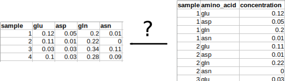
Are the different amino acid concentrations (glutamate, aspartate, glutamine and asparagine) different variables or are the column names actually different values of a variable amino_acid? The answer is that it depends on which analysis you want to do. If the analysis is the construction of a statistical model that predicts some property of the samples based on the concentrations of the different amino acids, then they are different variables. But if we want to make, for example, a stacked bar diagram that shows the amino acid composition for each sample then we have the second case. Fortunately, in such ambiguous cases you don’t have to choose beforehand because there are tools available in R with which we can easily convert one type of table into the other. We will discuss these in Chapter 11.
Repairing data
Sometimes it is obvious (or you believe it is obvious) that an error is present in the raw data. For example, somebody apparently reported lengths in centimeters but others in meters in the same column. In such a case you may want to repair the data. When doing this, you should always leave the original raw data files untouched, and create a new file with the repaired data in a folder called repaired_data, for example. The main reason is that you may be wrong, or others analyzing the same original data may wonder why your results differ from theirs. Repairing the original file would wipe out all records of the original data, and it would become unclear where mistakes and repairs were made. Keeping the original data and creating an additional repaired copy of the data implicitly records what you did. To be even more clear about this process you can document your repair actions. This can be done by adding comments about the repair actions or, if feasible, by writing a small script that repairs and saves the repaired copy of the data. If you write a paper or report these repair actions have to be referred to in the methods section, for example. A powerful tool that helps detecting and repairing complicated errors and inconsistencies in very large data sets, and that keeps a record of all the repair actions is OpenRefine.
7.2 Exercise
Exercise 1.
Carry out the exercise “Improving Messy Data” from the Data Carpentry for Biologists website. With “tidy data” the authors mean data organised as defined by the set of rules above.