17  Classifiers

A classifier is a statistical model, using a function that yields a class label or a distribution over class labels as its output. Many classifiers are capable of producing both types of output. Classifiers are used when the dependent or response variable is a class label, or in R-terms, when the response variable is a factor. The following are examples of the output of a classifier:

Class labels:

• Male (levels: Male, Female)
• Malignant (levels: Malignant, Benign)
• Iris versicolor (levels: Iris setosa, Iris virginica, Iris versicolor)

Distributions over class labels:

• Male: 0.9, Female: 0.1
• Benign: 0.05, Malignant: 0.95
• Iris setosa: 0.01, Iris virginica: 0.24, Iris versicolor: 0.75
• Iris setosa: 0.01, Iris virginica or Iris versicolor: 0.99

Distributions over class labels can be interpreted as probabilities. The first example would tell us that the probability that the person is a man is 90%, and that it is a female is 10%. The requirement for these distributions to be proper probabilities is that the numbers add up to 1.

17.1 Two main types of classifiers: discriminative and generative

We distinguish two main types of classifiers namely discriminative and generative classifiers. The main difference between these types is that generative models describe the entire joint distribution \(P(Y,X_1, \ldots, X_n)\) of predictor and response variables, whereas discriminative models only describe the conditional probabilities \(P(Y|X_1, \ldots, X_n)\). In practice, this means that generative models require much more information to become accurate. But they also enable the generation of new data similar to the training data by sampling from the distribution¹. Furthermore, in principle, you can also calculate p-values of new observations using the distribution a s anull hypothesis. Generative models, implicitly or explicitly, apply knowledge or assumptions about the processes that generate the joint distribution; they are models of the data generating process. The more assumptions or hypotheses you make about this process, the less data you need to specify such a model. In the example of the Naïve Bayes classifier, which is of the generative type, we will see that the problem of estimating \(P(Y,X_1, \ldots, X_n)\) is simplified by the assumption of conditional independence of the different predictors when conditioned on the response.

Logistic regression is a classifier of the discriminative type, usually applied when there are two levels in the response variable, yielding a distribution over the two levels. It is discussed in Section 17.2. Another type of classifier, the Naïve Bayes classifier is of the generative type and is discussed in Section 17.3. Both are are easy to understand and are representative of more complicated types of classifiers.

17.2 Logistic regression

Logistic regression functions are functions that yield a distribution over class labels as an output. Logistic regression is typically used in classifications with two alternatives, i.e. when the response variable has two levels.

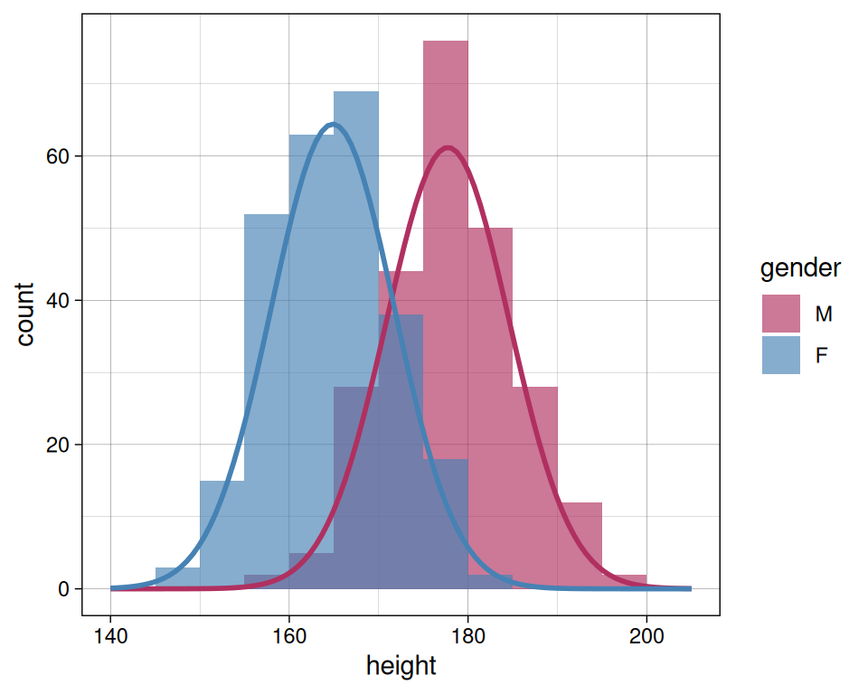
We start with the example that we saw before (Chapter 15), the bodymetrics data set bodymetrics.tab in the folder linearmodels. It contains measurements of height, weight and age of approximately 500 males and females. Suppose that instead of wanting to predict the height from the gender, we want to do it the other way around: predicting gender from height. Let’s make a histogram of the height differentiated by gender to see what the possibilities are:

Figure 17.1: Histogram of body heights, using a bin width of \(5\) cm

In this histogram I also added a smoothed version of the height distributions for both sexes. These are normal distributions with different means, but having equal variance² (and hence, equal standard deviation). Using either the counts in the bins or the heights of the smoothed distributions we can calculate the probability that a person with a certain body height is a man or a woman. Let’s call the probability that a person with body height height=\(x\) is a male \(P(S=\text{male}|H=x)\), or abbreviated \(P(m|x)\). Then the probability that this person is a female equals \(1 - P(m|x)\). In the figure below I have plotted the probability \(P(m|x)\) calculated by using the binned counts from the histogram as well as the smoothed distributions. It is simply the height of the male bin divided by the sum of the male and female bin, or the value of the density function for males divided by the sum of density functions of males and females.

Figure 17.2: The same histogram as above. The probability \(P(m|x)\) that the person is a man at the given height \(x\) is added, either calculated from the histogram bins (red dots) or from the smoothed distributions in figure above (blue line).

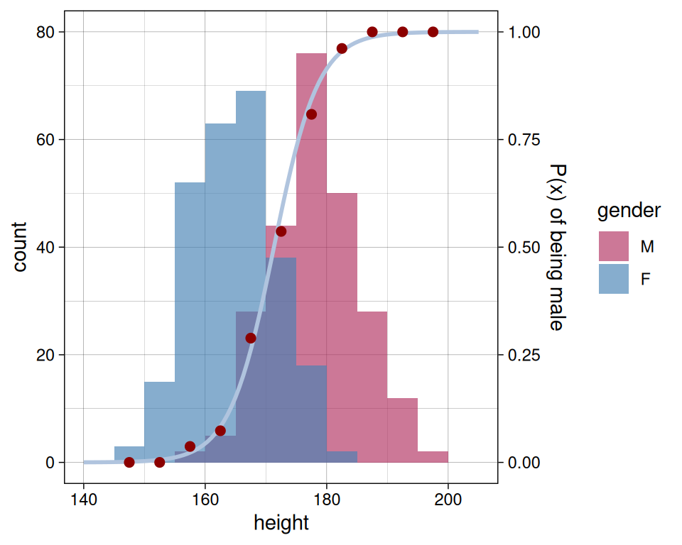
Having these estimations of the probability \(P(m|x)\) It would be straight-forward to make a classifier based on the predictor height (\(x\)): if the probability \(P(m|x) > 0.5\) then the label is ‘m(ale)’, otherwise, when \(P(m|x) \leq 0.5\), the label is ‘f(emale)’. Linear discriminant analysis (LDA) works exactly in this way: it obtains a description of the probability \(P(m|x)\) from smoothed normal distributions of the individual classes. However, there is another approach of obtaining a function \(P(m|x)\), which is used by logistic regression. To see how it works, we need the concept of odds³. The odds is the ratio \(\displaystyle \frac{P(m|x)}{1-P(m|x)}\), or how much more likely the person is a male than a female. This ratio equals \(1\) when the person is equally likely to be a man or a woman. In Figure 17.2 we can see that \(P = 1 - P = 0.5\) at a height of a little more than \(170\) cm.

Rather than using the odds itself, it is common to use its natural logarithm also called the log-odds

\[ \ln{\left(\frac{P(m|x)}{1-P(m|x)}\right)} \tag{17.1}\]

The function

\[ l(p) = \ln{\left(\frac{p}{1-p}\right)} \tag{17.2}\]

is called the logit function. Logistic regression is based on the fact that something peculiar happens if we transform the probability \(P(m|x)\) with the logit function to \(l(P(m|x))\). This is shown below for the values of \(P(m|x)\) calculated from the smoothed distributions:

Figure 17.3: Logit transform of probability \(P(m|x)\) as calculated from the smooth distributions plotted as a function of the body height \(x\).

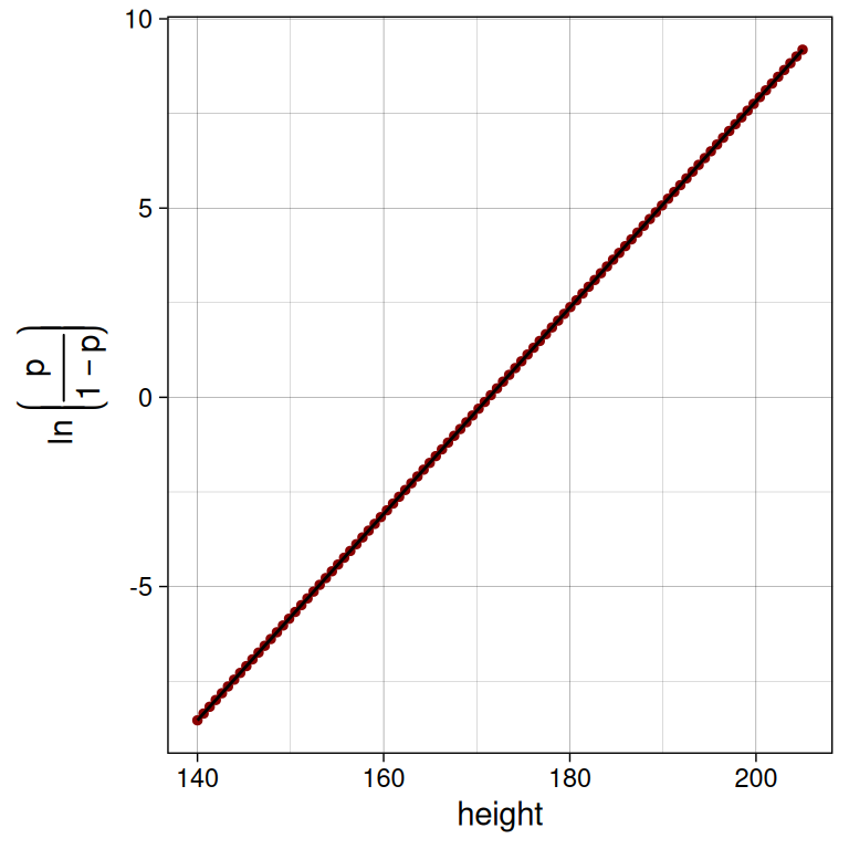
As you will guess, this perfectly straight line is not a coincidence. This is what you get if you use two normal distributions with equal standard deviation but different means to model the underlying distributions. The slope of this line will be steeper when the two distributions have less overlap, and the point where it passes through the \(x\)-axis (around height=171) is the point of equal odds. Logistic regression uses this fact. If apparently we can fit the log-odds by a straight line \(f(x) = \beta_0 + \beta_1 x\):

\[ \ln{\left( \frac{P(m|x)}{1-P(m|x)} \right) } = f(x) \]

then let’s find out how \(P(m|x)\) itself can be modeled as a function of \(x\):

\[ \begin{align*} \frac{P(m|x)}{1-P(m|x)} &= e^{f(x)} \\ P(m|x) &= e^{f(x)} - e^{f(x)} \cdot P(m|x) \\ P(m|x) \left( 1 + e^{f(x)} \right) &= e^{f(x)} \\ P(m|x) &= \frac{e^{f(x)}}{1 + e^{f(x)}} = \frac{1}{1 + e^{-f(x)}} \end{align*} \tag{17.3}\]

Equation 19.1 is called the logistic equation. This is the function that is used in logistic regression to fit \(P(m|x)\) to the data.

17.2.1 Logistic Regression: a case of Generalized Linear Modeling

Logistic regression is a special case in a framework of more general modeling techniques called Generalized Linear Modeling or GLM. In contrast to ordinary linear models, generalized linear models have two modifications:

1. The response variable \(y\) does not have to be normal-distributed, and it does not have to be a continuous variable. It could, for example, be a count variable with Poisson or Binomial distribution.
2. A linear function of the predictor variables is transformed through a non-linear, so-called link function to fit the sampled response variable.

The second modification needs some explanation. In statistical modeling we predict parameters of a probability distribution of the response variable rather than the response variable itself, often their mean. In linear modeling, since the underlying distribution is assumed to be the normal distribution, the predicted mean \(\mu\) is the expected value of the response variable itself. However for other distributions these parameters do not have to correspond to the mean.

For example, in logistic regression, the random variable can only have two values, 0 or 1⁴. The variable \(y'\) is Bernoulli-distributed (Chapter 14). The Bernoulli distribution has a single parameter, \(\theta\), which is the probability that the outcome of a single draw will equal 1. In logistic regression, we estimate how this parameter \(\theta\) depends on a predictor variable \(x\). In fact, we model \(\theta(x)\).

The link function referred to above is, for the case of logistic regression, the logit function \(l\) in eq Equation 17.2. The logit function links the parameter of the distribution that we want to predict to a linear function of the predictor variable(s). Here, it maps the interval of \(\theta\), \([0,1]\), to the entire set of real numbers, the co-domain of the linear function.

Fitting of GLM’s, in contrast to ordinary LM’s or non-linear models with normal-distributed response variables, is not carried out by minimizing the sum of squared residuals. The reason is that least-squares does not yield unbiased estimates if the response variable is not normal-distributed. To fit a GLM, a technique called likelihood maximization (see Chapter 19) is used. For normal-distributed response variables, likelihood maximization coincides with minimization of the sum of squared residuals. This does not hold for other distributions.

17.2.2 Logistic regression in R

In R we perform logistic regression using the glm() function for generalized linear modeling. This function is part of the standard stats package which is loaded at the start of R. The function can be called in the same way as the lm() function for the example of predicting gender from body height:

log.fit <- glm(gender ~ height, data=bodymetrics, family='binomial')

The argument family='binomial' tells the algorithm that the response variable has a binomial distribution⁵. The fitted function \(\theta(x)\) looks as follows:

Figure 17.4: Logistic regression of the bodymetrics data using the gender as the response variable and height as the predictor variable. The vertical red line is the divide between the probability of being male larger or smaller than \(0.5\).

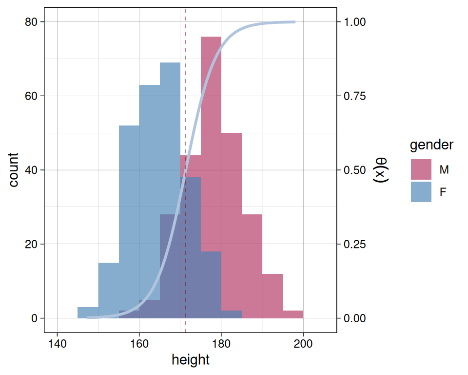
The fit has the following coefficients for the function \(f(\text{height}) = \beta_0 + \beta_1 \text{height}\)

• \(\beta_0 = 46.8\)
• \(\beta_1 = -0.273\)

So, the fitted linear function \(f(x)\) equals the log-odds of the probability that the person is a man. This is equal to 0 if \(P = 1-P = 0.5\), and it is \(>0\) if the probability that the person is a man is larger than that the person is a woman. The fitted \(f(\text{height})\) equals zero when \(\text{height} = -\frac{\beta_0}{\beta_1} = 171\) cm. A vertical line is drawn at this position in Figure 17.4. Although we estimate the probability \(P(m|x)\), the fitted model can also be simplified to become a true classifier by using the rule:

\[ S = \begin{cases} \text{male} & \text{if } P(m|x) \geq 0.5 \\ \text{female} & \text{if } P(m|x) < 0.5 \end{cases} \] which is equivalent to

\[ S = \begin{cases} \text{male}, & \text{if } x \geq - \beta_0 / \beta_1 \\ \text{female}, & \text{if } x < - \beta_0 / \beta_1 \end{cases} \]

One way to assess the goodness of fit of this classifier is to make a confusion matrix, a table that tells you per level of the response variable how well the classifier predicted the training data:

>      prediction
> truth   M   F
>     M 202  45
>     F  44 216

This shows that the prediction for males and females is approximately equally accurate, and that the overall accuracy equals 82%, which is fair, but not very good (1 in 5 is false). Can it be improved?

We have other predictors as well, namely weight and age, and there is no reason to not add them to the linear predictor equation:

\[ f(x) = \beta_0 + \beta_1 \text{height} + \beta_2 \text{weight} + \ldots \]

Let’s add weight:

log.fit2 <- glm(gender ~ height + weight, data=bodymetrics, family='binomial')

This yields the following confusion table:

>      prediction
> truth   M   F
>     M 210  37
>     F  38 222

with an overall correct prediction of 85%. This is a little better than before but not much. We could have expected this, because it appeared earlier that height and weight are highly correlated, indicating that if you know one, the other doesn’t yield much more information.

17.3 Naïve Bayes classifiers

We treat the Naïve Bayes classifier because it is a classifier that is popular and used often in classification tasks. Once you have internalized Bayes Law, the method is also easy to understand. Despite its simplicity and the simplifying assumptions behind it, the Naïve Bayes Classifier is very successful in many classification tasks. We explain the classifier using an example.

17.3.1 A crime scene

At a conference for members of boards of directors a murder has taken place: the head of a company has been shot in his hotel room. The window to his room, located on the ground floor, is open. Those arriving at the scene immediately after hearing the shot perceived a hint of perfume in the room. The police found a footprint, belonging to the murderer, in the flower bed below the window. The foot size was 24.3 cm. Since the conference hotel was at a strictly guarded site, only a conference participant could be the murderer. The police wants to know whether, based on current evidence, it is more likely that a man or a woman was the murderer.

We are going to use a Naïve Bayes classifier to solve this problem. We are told that a person has a particular foot size. What does this tell us about the gender of this person? If there is a correlation between foot size and gender, then the variable foot size carries information about the variable gender. We know from experience that such a correlation exists. If the footprint size is small, it tells us that the chance that it belongs to a woman is larger than that it belongs to a man, since in the entire population, women have small foot sizes more often than men. We were also told that the murderer wears perfume. This gives information about the gender if there is a difference in the fraction of men or women that wear perfume. How can we combine these two pieces of information to a single number that tells us whether it is more likely that the person is a woman or a man?

17.3.2 Applying Bayes rule

perfumed	male	female
yes	0.1	0.35
no	0.4	0.15

The joint probability distribution for the two variables gender and perfumed (wearing perfume) is summarized in the table to the right. We will abbreviate the variable gender by \(G\) and perfumed by \(P\). This table allows us to calculate \(P(P|G)\) for the general population. We know that the murderer wears perfume, and we want to know the probability \(P(G|P=\text{yes})\). We know that Bayes rule (Chapter 14) relates the conditional probability \(P(G|P)\) to \(P(P|G)\). Now we can calculate \(P(G|P=\text{yes})\) as follows:

\[ P(G|P=\text{yes}) = \frac{P(P=\text{yes}|G) \cdot P(G)}{P(P=\text{yes})} \]

In which we should substitute for \(P(G)\) not the distribution of gender in the general population, but the gender distribution in the board of directors! In the language of Bayesian statistics, \(P(G)\) is also called a prior probability and \(P(P=\text{yes}|G)\) is called a likelihood. Here \(P(G=\text{m})\)=0.80 and \(P(G=\text{f})\)=0.20. We assume that among men and women in boards of directors, the use of perfume is similar to that in the general population, i.e. the likelihoods \(P(\text{P}|G)\) are the same as in the general population, namely 70% of the women wears perfume and 20% of the men. You take a member of this population and observed that he or she uses perfume (\(P=\text{yes}\)).

If we consider this population, the board of directors, then what are the odds that this person is a man or a woman? For a man this probability is

\[ P(G=\text{m} | P=\text{yes}) = \frac{P(G=\text{m}) \cdot P(P=\text{yes}|G=\text{m})}{P(P=\text{yes})} = \frac{0.80 \cdot 0.20}{P(P=\text{yes})} = \frac{0.16}{P(P=\text{yes})} \]

and for a woman it is

\[ P(G=\text{f} | P=\text{yes}) = \frac{P(G=\text{f}) \cdot P(P=\text{yes}|G=\text{f})}{P(P=\text{yes})} = \frac{0.20 \cdot 0.70}{P(P=\text{yes})} = \frac{0.14}{P(P=\text{yes})} \]

We do not have to calculate the marginal probability \(P(P=\text{yes})\) to be able to conclude that \(P(G=\text{m} | P=\text{yes}) > P(G=\text{f} | P=\text{yes})\), because we divide both expressions above by the same \(P(P=\text{yes})\). Hence, based on the information about the perfume it is more likely that the murderer is a man than a woman.

17.3.3 Choosing the class

The previous calculation demonstrates how we could use prior and likelihood distributions to make a decision about the gender classification of this person. The rule, called maximum a posteriori rule or MAP rule, is that we choose that value for gender that maximizes the conditional probability \(P(G|P=\text{yes})\), hence the value for gender that maximizes the numerators calculated above. Since

\[ P(G=\text{m}|P=\text{yes}) \varpropto 0.80 \cdot 0.20 = 0.16 \]

and (\(\varpropto\) means: “is proportional to”)

\[ P(G=\text{f}|P=\text{yes}) \varpropto 0.20 \cdot 0.70 = 0.14 \]

using the MAP rule we would classify the murderer as a man. It is not a very convincing case though, because the values do not differ very much. We say that the odds for a man are a factor \(\frac{0.16}{0.14} = 1.14\). Concluding: given only the observation of perfume, and the proportion of men among boards of directors, we would, using a Bayes classifier, decide that the murderer is likely to be a man.

17.3.4 Continuous predicting variables

\(P\) or perfumed is a discrete variable, a factor in R terminology. How do we carry out the same analysis with a continuous variable like foot size? And furthermore, how do we combine this information with information about wearing perfume to decide on the gender classification of the murderer? We treat these two problems one by one.

Previously we knew the conditional distribution \(P(P|G)\), or the likelihood as it is also called, by reading it from the table of joint probabilities of all combinations of values of gender and perfumed in the general population. Now, we need to have information about the continuous distribution of foot sizes specified separately for men and women in the general population, i.e. we need probability density functions \(f\) of foot size conditional on gender. Suppose that foot sizes are normal-distributed with means \(\mu_m\) and \(\mu_f\) and standard deviations \(\sigma_m\) and \(\sigma_f\). We have measured these means and standard deviations in the general population and assume that they are valid for boards of directors as well. Then, abbreviating the variable foot size as \(F\), we have

\[ f(\text{F}=s | G=\text{m}) = \frac{1}{\sqrt{2 \pi \sigma_m^2}} e^{\left(\frac{s-\mu_m}{2 \sigma_m}\right)^2} \]

and

\[ f(\text{F}=s | G=\text{f}) = \frac{1}{\sqrt{2 \pi \sigma_f^2}} e^{\left(\frac{s-\mu_f}{2 \sigma_f}\right)^2} \]

For a population in which \(\mu_m\)=26.9, \(\mu_f\)=24.2, \(\sigma_m\)=1.4 and \(\sigma_f\)=1 these would look like the figure below.

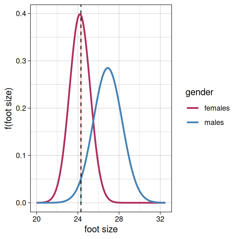
The police observed that foot size=24.3 (black dashed line). We could make a decision rule that is based on the conditional density functions, namely that whichever density is larger at the given size corresponds to the gender that we choose to be most likely. We should note that probability density \(f(F|G)\) is not a probability! We get a probability from a probability density function by integrating over a piece of the variable foot size. However, the probability density at foot size=24.3” is virtually proportional to a tiny integrated interval around this value (the colored areas). Therefore, we can use both probability density functions to obtain values that are proportional to the conditional probabilities of observing foot sizes close to 24.3. Having 80% of men again as marginal probability, we get

\[ P(G=\text{m}|F=24.3) \varpropto f(F=24.3|G=\text{m}) \cdot 0.80 = 0.041 \]

and

\[ P(G=\text{f}|F=24.3) \varpropto f(F=24.3|G=\text{f}) \cdot 0.20 = 0.079 \] In this case we would decide that the murderer is a woman. And this piece of evidence is a little more conclusive because the odds for a woman rather than a man being the murderer are \(1.954\).

Note

Using Gaussian probability density functions to model the distributions of foot size is only one way of modeling a distribution. Many other standard distributions can be applied in naïve Bayes classifiers. You can use whichever distribution best fits the real distribution, or accommodates your well-founded ideas about it. Modeling and smoothing of data is particularly important if the number of training samples is small compared to the sampling space, as is clearly the case with continuous variables. You can find a few examples of distribution models used in naive Bayes classifiers in Wikipedia.

17.3.5 Combining information from different predictor variables

How do we combine the two pieces of information about the variables perfumed and foot size to decide whether the murderer is a man or a woman? We know the variables \(P\) and \(F\) and we want to infer what this means for the variable \(G\), hence we want to calculate the conditional probability distribution \(P(G|P,F)\). Using a Bayes rule for multiple variables we can express it in terms of the conditional probability distribution \(P(P,F|G)\) and the marginal probability \(P(G)\):

\[ P(G\,|\,P,F) \propto P(P,F\,|\,G) \cdot P(G) \]

The problem is that we do not know the joint conditional probability distribution \(P(P,F|G)\) for the general population. The only distributions that we know are \(P(P|G)\) and \(P(F|G)\). However, if we assume that the latter two are conditionally independent, i.e \(P(P,F|G) = P(P|G) \cdot P(F|G)\), then this simply becomes

\[ P(G\,|\,P,F) \propto P(P\,|\,G) \cdot P(F\,|\,G) \cdot P(G) \] This assumption of conditional independence of the predictor variables is what Naïve Bayes gave its name. It is somewhat naïve to assume that these variables will be conditionally independent. The corresponding graphical model for the naïve assumption is shown in Figure 17.5.

Figure 17.5: Conditional independence assumption of perfumed and foot size.

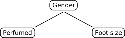
The naïve assumption considerably simplifies the task of estimating the joint conditional distribution \(P(P,S|G)\). Instead of having to estimate a two-dimensional distribution \(P(P,F|G)\) for every value of \(G\), we approximate this distribution by multiplying two one-dimensional distributions \(P(P|G)\) and \(P(F|G)\). This becomes a dramatic reduction of complexity when the number of predictor variables is large and when one or more of these are continuous variables. Then it is practically impossible to properly sample the space of all combinations (all dimensions) of predictive variables.

Figure 17.6: The naïve assumption behind the Naïve Bayes classifier. There are no other links between the predictors than the ones running via the response variable, i.e. all pairs of predictors are independent, conditional on the response.

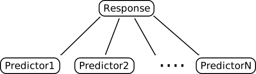
In general, the naïve assumption allows us to quantify the odds having only information about the one-dimensional conditional probability distributions \(P(\text{Predictor}_i | \text{Response})\).

Let’s see what we get when combining the two pieces of information, \(F=24.3\) and \(P=\text{yes}\).

\[ P(G=\text{m}|F=24.3, P=\text{yes}) \varpropto f(F=24.3|G=\text{m}) \cdot 0.20 \cdot 0.80 = 0.0081 \]

and

\[ P(G=\text{f}|F=24.3, P=\text{yes}) \varpropto f(F=24.3|G=\text{f}) \cdot 0.70 \cdot 0.20 = 0.0556 \]

which, using the MAP rule, leaves us no other option than to conclude that the murderer was a woman with an odds factor \(6.84\)!

Surprisingly, the odds factor shows that this becomes a much more convincing case than when studying either of the single pieces of evidence individually! However, we should note that the numerical correctness of this odds factor may strongly depend on the correctness of the naïve assumption! The naïve assumption of conditional independence of the observed variables seems reasonable in case of variables foot size and perfumed. However, there are cases where it is clearly incorrect. For example, suppose that we also observe the variable shoe brand (\(B\)), from the imprint of a shoe sole. The probability of observing a certain shoe brand will not only depend on the gender, the variable that we want to predict, but also on the foot size. This is the case if certain shoe brands only produce small sizes for males, for example Italian brands. If you know that you’re dealing with a man, then knowing his foot size gives you additional information about the probability of observing this particular brand! Therefore, contrary to the conditional independence assumption \(P(B|F,G) \neq P(B|G)\)! Nevertheless, it has been demonstrated several times that naïve Bayes classifiers perform surprisingly well, even when the assumption of conditional independence of observed predictor variables is clearly incorrect. Below we will see an example of that case. One of the reasons is, of course, that we do not use the exact numerical outcome of the likelihood product, or the conditional probability itself, but we only want to know which one is largest. This gives the method a certain robustness against violation of the assumption of conditional independence. Another reason is that, because of the simplicity of the model (due to conditional independence we use much less parameters to fit the probability distribution that models the data), it is quite insensitive to over-fitting.

Important

Please make sure that you understand the difference between “independence of variables” and “independence of variables conditioned on an other variable”. For example, the naïve assumption which says that “foot size” and “perfumed” are independent conditioned on gender, does not mean that “perfumed” and “foot size” are independent. They clearly are not! People with small foot sizes use perfume more often. However, what it means is that when we look at the subpopulation of men only, we do not expect a relation between “foot size” and “perfumed”, nor do we expect such a relation when we look at women only. In other words, the correlation between foot size and perfumed is fully explained by the gender. Also see exercise 6 below.

17.4 Exercises

17.4.1 General questions

Exercise 1. Generative and discriminative models

a. Having the data from Figure 17.1, how would you estimate a p-value to test the null hypothesis that a person is a man? Why is it not possible to calculate that p-value with our model of \(P(m|x)\)?

Answer

We could model the distribution of heights of males by a suitable distribution like the normal distribution. Then we could calculate the probability that athe observed height or a lower value was drawn from this distribution.

To calculate a p-value we need the distribution \(P(x|m)\), but we have modeled \(P(m|x)\). Clearly we could calculate one from the other using Bayes rule, but for that we additionally need the marginal distributions \(P(x)\) and \(P(m)\), which were not modeled.

b. Show how it is possible to calculate the full joint distribution \(P(G,P,F)\) from the modeled conditional probabilities \(P(P|G)\), \(P(F|G)\) and the marginal distribution \(P(G)\).

Tip

Use Bayes rule as well as the naïve Bayes assumption.

Answer

\[ \begin{align} P(G|P,F) &= \frac{P(P,F|G) \cdot P(G)}{P(P,F)} \\ &= \frac{P(P|G) \cdot P(F|G) \cdot P(G)}{P(P,F)} \\ P(G|P,F) \cdot P(P,F) &= P(P|G) \cdot P(F|G) \cdot P(G) \\ P(G,P,F) &= P(P|G) \cdot P(F|G) \cdot P(G) \end{align} \]

Metagenome analysis is often performed by sequencing of 16S ribosomal RNA. Using databases of these sequences it is possible to assign such sequences to different species, providing a way to characterize a microbiome, for example. Often you will find rare point mutations in the sequences. The question is then often: is this a real sequence difference, or is it an artifact perhaps caused by the PCR amplification step used in the experiment? The DADA algorithm (Rosen et al., 2012) tries to solve this question. The algorithm classifies an observed point mutation as real or artifact.

c. Read the Background section in the paper and indicate whether the DADA classifier uses a discriminatory or generative type of model. Indicate why you think this is the case.

Answer

It uses a model of the data generating process and calculates p-values for observing a mutation a number of times under the null hypothesis that it is a PCR artifact. Therefore, it uses a generative-type model.

17.4.2 Logistic regression

Exercise 2. Identifying lung tumor tissue

The expression of genes in healthy lung tissue and from lung tumors was measured in 107 tissue samples. The file lung_tumor_expression.csv in the folder logistic contains the expression values for two genes, ATP1A2 (encodig the ATPase Na+/K+ transporting subunit alpha 2) and KDELR2 (encoding the KDEL endoplasmic reticulum protein retention receptor 2), that were selected because they are differentially expressed in healthy and tumor tissues. The goal of this exercise is to make a classifier for healthy and tumor tissue based on these expression values.

a. Read the data into a data frame

Answer

require(tidyverse)
d <- read_csv(file.path(webserver, 'logistic', 'lung_tumor_expression.csv')) |>
  mutate(tissue = as.factor(tissue), sample = as.factor(sample))

d.long <- d |>
  pivot_longer(cols = c(ATP1A2, KDELR2), names_to = 'gene', values_to = 'expression') |>
  mutate(gene = as.factor(gene))

head(d)

> # A tibble: 6 × 4
>   tissue     sample    ATP1A2 KDELR2
>   <fct>      <fct>      <dbl>  <dbl>
> 1 Lung Tumor GSM254625   5.21   11.6
> 2 Lung Tumor GSM254627   5.87   10.8
> 3 Lung Tumor GSM254629   5.87   10.4
> 4 Lung Tumor GSM254630   5.40   10.5
> 5 Lung Tumor GSM254631   5.91   11.4
> 6 Lung Tumor GSM254633   5.52   11.8

b. Make two boxplots of the expressions of both genes as a function of the tissue type. Which of the two provides the best discrimination between the two types of tissue?

Answer

ggplot(d.long, aes(x = tissue, y = expression)) +
  geom_boxplot() +
  facet_wrap(~ gene, scales = "free")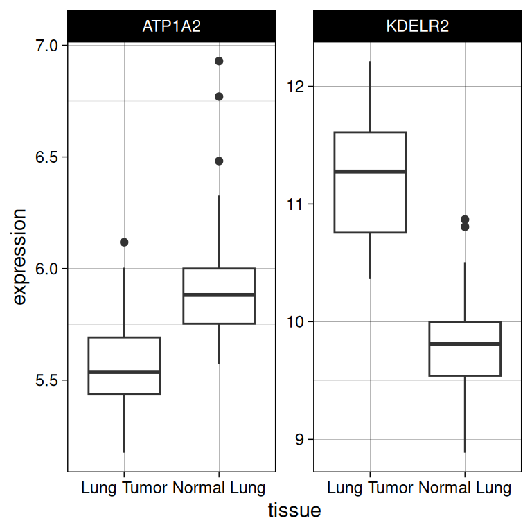

The gene KDELR2 provides the best discrimination between the two tissue types

c. Use the gene with the best discrimination to do a logistic regression. Make a confusion matrix of the prediction, and give the fraction of correct predictions.

Answer

log.fit1 <- glm(tissue ~ KDELR2, data = d, family='binomial')
d$prediction1 <- ifelse(predict(log.fit1) < 0, 'Lung Tumor', 'Normal Lung')
correctfraction <- sum(d$tissue == d$prediction1)/nrow(d)
table(d[c('tissue', 'prediction1')])

>              prediction1
> tissue        Lung Tumor Normal Lung
>   Lung Tumor          56           2
>   Normal Lung          4          45

The fraction of correct predictions is 0.94.

d. Can you improve the predictor by adding the expression values of the other gene in the model?

Answer

log.fit2 <- glm(tissue ~ KDELR2 + ATP1A2, data = d, family='binomial')
d$prediction2 <- ifelse(predict(log.fit2) < 0, 'Lung Tumor', 'Normal Lung')
correctfraction <- sum(d$tissue == d$prediction2)/nrow(d)
table(d[c('tissue', 'prediction2')])

>              prediction2
> tissue        Lung Tumor Normal Lung
>   Lung Tumor          56           2
>   Normal Lung          4          45

The fraction of correct predictions remains the same, so the expression data of the gene ATP1A2 does not improve the model.

17.4.3 Naive Bayes

Exercise 3. Predicting iris species

Below is a small sample of the iris data:

>     Sepal.Length Sepal.Width Petal.Length Petal.Width    Species
> 14           4.3         3.0          1.1         0.1     setosa
> 43           4.4         3.2          1.3         0.2     setosa
> 51           7.0         3.2          4.7         1.4 versicolor
> 68           5.8         2.7          4.1         1.0 versicolor
> 85           5.4         3.0          4.5         1.5 versicolor
> 129          6.4         2.8          5.6         2.1  virginica

Here we have a variable, Species, that we want to predict. It has three levels: setosa, versicolor, virginica. The predictor variables are all continuous valued. We will split the data in a training set, from which we will construct the “likelihood” and “prior” distributions, and a test set on which we will apply our classifier. In the “board of directors murder” example, we estimated the likelihood distributions (concerning the use of perfume and foot size) from the general population of human beings, and adapted the prior (male/female) distribution to what we knew about it for boards of directors. Here we will estimate these from the training set.

a. Make two index vectors, trainset and testset that can be applied, using a construct like iris[trainset,], to split the iris data frame into a set of training samples (80% of the data) and a set of test samples (20%). Use a random selection of the data to make the split. Then split the data.

Answer

trainset <- sample(rownames(iris), size=trunc(0.8*dim(iris)[1]))
testset <- rownames(iris)[!(rownames(iris) %in% trainset)]
trainsamples <- iris[trainset,]
testsamples <- iris[testset,]

Note: from here on, there are two ways of carrying out this exercise: building a classifier using your own functions, as suggested in questions b-d, or by using the naiveBayes() function from the e1071 package and pick up at question e. To build the classifier yourself you need somewhat advanced mastering of the R language (or: you obtain this craftsmanship by building it yourself).

b. Calculate an 1 \(\times\) 3 array of priors from the test set (you know, the expected fractions of each of the three species), or make a prior based on your belief of what fractions you could expect. The columns should carry the species names.

Answer

# Either calculate a prior:
prior <- tapply(
  rep(1/length(trainsamples$Species), length(trainsamples$Species)),
  trainsamples$Species, sum)
# Or make one based on your belief of the distribution:
prior <- array(1/3, dim=3, dimnames=list(levels(iris$Species)))

c. Calculate means and standard deviations of the four predictor variables for each of the species using the training set. We will need these to model their distributions conditional on species using normal distributions. Put the means and standard deviations in a list, where each element corresponds to a predictor variable and consists of matrices with three rows (corresponding to the species) and two columns (corresponding to the mean and standard deviation conditioned on species). Below you will find out why such a list is a convenient arrangement of the data.

Tip

Use a tapply nested in an lapply to generate a list containing for each of the predictor variables a list of vectors of mean and standard deviations conditional on Species. Use tapply as shown in the exercises in the chapter about Vectorization. Subsequently, put the inner lists in a matrix using cbind() called with do.call().

Answer

nb <- lapply(
  apply(trainsamples[1:4], 2, function(x){
    tapply(x, trainsamples[[5]], function(x){
      c(mean(x),sd(x))})}
    ),
  function(x){do.call(rbind,x)}
)

Explanation: The code consists of two nested apply-like functions. The outer part (lapply) loops over each of the predictor columns and sends it to the inner function. The inner part calculates the mean and standard deviation of that column split by species (using the fifth Species column) and puts it in a vector (mean, stdev).

To be able to calculate a Gaussian probability density below, we need a function that takes a value, a mean and a standard deviation and returns the corresponding probability density. The standard dnorm() function seems to do this exactly.

d. Now comes a difficult part. For each sample in the test set you have to calculate the dnorm() using the list constructed above.

Answer

posteriors <- t(
  apply(testsamples[1:4], 1,
       function(y) {
         apply(
           sapply(names(y),
                  function(varname) {
                    apply(nb[[varname]], 1, function(x) {
                      dnorm(y[[varname]],x[1],x[2])
                      }
                    )
                  }), 1, prod)
      }))

head(posteriors)

>       setosa   versicolor    virginica
> 4  2.4803318 8.307170e-18 7.609501e-25
> 5  5.9182433 3.000193e-19 1.909509e-25
> 8  6.6834870 6.559654e-18 2.121275e-24
> 9  0.6506896 1.683882e-18 6.627489e-26
> 11 3.2105054 9.184281e-19 1.687805e-24
> 30 3.0458808 2.499539e-17 4.252524e-24

Explanation: The nested set of apply-like functions above looks quite complicated, but it solves the problem very effectively. How do you construct such a method? I started from the center, and asked: what if I have one variable from one row of the test set, how do I then calculate the conditionals?

varname <- "Sepal.Length" # for example
y <- testsamples[1,1:4] # first sample, for example

Then the following apply gives me a vector of conditional values for this variable:

apply(nb[[varname]], 1, function(x) {dnorm(y[[varname]],mean=x[1],sd=x[2])})

>      setosa  versicolor   virginica 
> 0.560563745 0.029557831 0.004685445

I need to calculate these conditionals for each predictor variable. So, I take a vector with the names of y (names(y)) and lapply the previous function to each of these names. I then get a list of conditionals containing an entry for each of the predictor variables:

lapply(names(y), function(varname) {
  # now the previous piece of code
  apply(nb[[varname]], 1, function(x) {dnorm(y[[varname]],x[1],x[2])})
  })

> [[1]]
>      setosa  versicolor   virginica 
> 0.560563745 0.029557831 0.004685445 
> 
> [[2]]
>     setosa versicolor  virginica 
>  0.7028728  0.6313132  1.1532346 
> 
> [[3]]
>       setosa   versicolor    virginica 
> 2.078731e+00 9.603597e-08 2.628332e-13 
> 
> [[4]]
>       setosa   versicolor    virginica 
> 3.028376e+00 4.635555e-09 5.358058e-10

I get a list of vectors with the same length! Using sapply instead of lapply would “simplify” this list of vectors to a matrix, which is easier to use in the subsequent step:

sapply(names(y), function(varname) {
  # now the previous piece of code
  apply(nb[[varname]], 1, function(x) {dnorm(y[[varname]],x[1],x[2])})
})

>            Sepal.Length Sepal.Width Petal.Length  Petal.Width
> setosa      0.560563745   0.7028728 2.078731e+00 3.028376e+00
> versicolor  0.029557831   0.6313132 9.603597e-08 4.635555e-09
> virginica   0.004685445   1.1532346 2.628332e-13 5.358058e-10

For each of the posteriors, I need to calculate the product conditioned on species name, which means that I need to calculate the products per row of the previous matrix, using a construct apply(..., 1, prod). prod calculates the product of elements in a vector:

apply(
  # the previous piece of code
  sapply(names(y), function(varname) {
    apply(nb[[varname]], 1, function(x) {dnorm(y[[varname]],x[1],x[2])})
    }),
  1, prod)

>       setosa   versicolor    virginica 
> 2.480332e+00 8.307170e-18 7.609501e-25

Now this was for one row, y, of the test data. I now make a function of the previous piece of code and apply it to all rows in the testsamples data frame:

apply(testsamples[1:4], 1,
      function(y) {
        # the previous piece of code
        apply(
          sapply(names(y), function(varname) {
            apply(nb[[varname]], 1, function(x) {dnorm(y[[varname]],x[1],x[2])})
            }),
          1, prod)
      })

This gives the result with posteriors in rows and samples in columns. I want to have then in the transposed arrangement, so I transpose the previous matrix and get the desired result.

e. Make a prediction of the species for each flower in the test samples based on the likelihoods. Also calculate the fraction of correct predictions. Tip: use the max.col() function.

Answer

priors <- c(1/3,1/3,1/3)
predictions <- colnames(posteriors)[max.col(t(t(posteriors)*priors))]

correct <- sum(predictions==as.character(testsamples[[5]]))/length(predictions)

correct

> [1] 0.9333333

This shows that a naïve Bayes classifier performs very well on this data set.

f.
Is the naïve assumption valid for the predictor variables in the iris data set? Demonstrate why or why not.

Answer

No, it is not valid. For example, if we plot the petal width against the petal length then we see a clear correlation in the red points only.

plot(iris$Petal.Length, iris$Petal.Width, col=iris$Species, pch=19)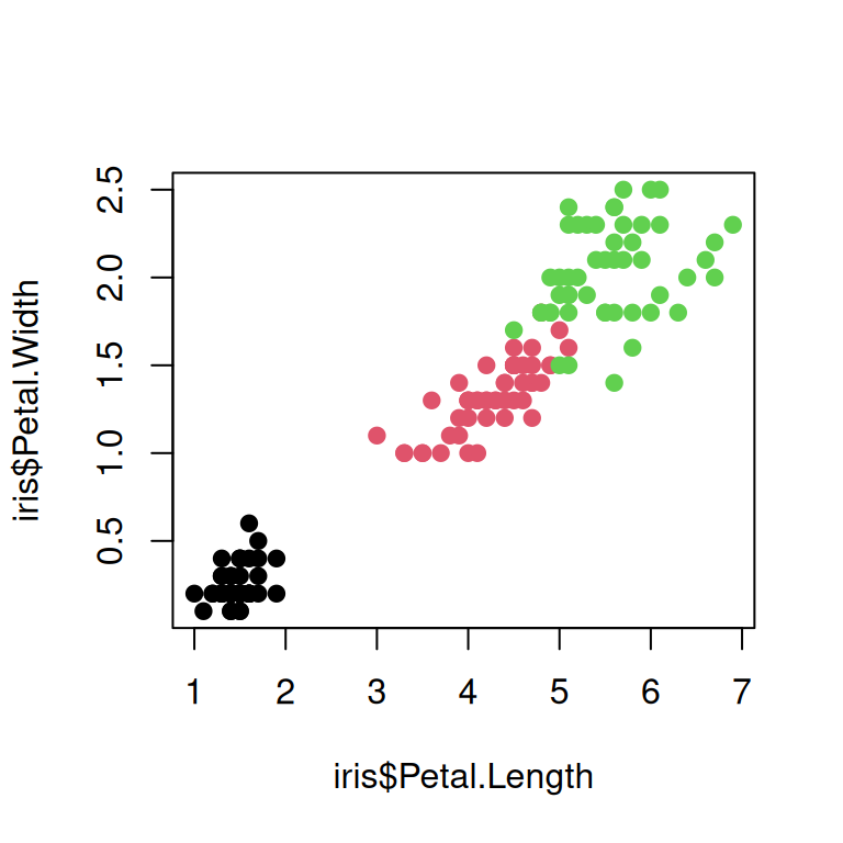

Or performing a two-sided Pearson product-moment correlation test yields a significant correlation for each species separately:

iris |> 
  group_by (Species) |>
  group_map(~tidy(cor.test(.x$Petal.Length,.x$Petal.Width))) |>
  bind_rows() |>
  mutate(species=levels(iris$Species), .before=estimate) |>
  select(species, estimate, statistic, p.value) |>
  flextable() |>
  colformat_double(j = c(2,3,4), digits=3)

species	estimate	statistic	p.value
setosa	0.332	2.435	0.019
versicolor	0.787	8.828	0.000
virginica	0.322	2.357	0.023

Clearly, both variables are correlated with species (which is why we can use them to identify the species). However, in contrast to the naïve assumption, we see that within each species both variables are also correlated.

Exercise 4. Predicting income

The adult data set contains census data from the american population. It also contains a column that says whether a person earns more or less than 50000 dollar per year. The goal is to predict the income from the other variables. The predictor variables are continuous and discrete (which is more advanced than the previous exercise). Instead of calculating model conditional distributions using your own code, use the naiveBayes() function from the e1071 package to do that. Split the data (80:20) in a training and a test set, and predict the income (more or less than 50K) from the model distributions. How well does your predictor perform?

Answer

library('e1071')
# loaded the data set in the data frame 'adult'
trainset <- sample(rownames(adult), size=trunc(0.8*dim(adult)[1]))
testset <- rownames(adult)[!(rownames(adult) %in% trainset)]
trainsamples <- adult[trainset,]
testsamples <- adult[testset,]
model <- naiveBayes(income~., data = trainsamples)
prediction <- predict(model, testsamples)
correct <- sum(prediction==as.character(testsamples[[15]]))/length(prediction)
correct # approximately 82% correct

Rosen, M.J., Callahan, B.J., Fisher, D.S. & Holmes, S.P. (2012) Denoising PCR-amplified metagenome data. BMC Bioinformatics, 13. https://doi.org/10.1186/1471-2105-13-283.

---

1. You may have heard of the fact that ChatGPT is a generative language model. You can generate new data (text) with it which is similar to data that was used to train it.

2. Means and variance were calculated from the data

3. Odd: in 16-th century England an “amount by which one thing exceeds or falls short of another”, but see, in the online etymology dictionary, its origin from the Norse oddi and strange development in that language from a word that is related to dutch and german oord or Ort (point, place). Odd is truly odd.

4. If the original random variable has two character labels, like ‘M’ and ‘F’, then these are first converted to a new variable \(y'\) that has the values \(0\) or \(1\).

5. Actually, a Bernoulli distribution.