8 Matrix notation – Math for BSB

8.1 A notation for systems of linear equations

We now introduce matrix notation, a concise way to write systems of linear equations. For example, consider:

\[ \begin{align*} 2x-3y & = 2\tfrac{1}{2} \\ x+4y & = 4 \end{align*} \]

In matrix notation, this system becomes:

\[ \begin{bmatrix} 2 & -3 \\ 1 & 4 \end{bmatrix} \begin{bmatrix} x \\ y \end{bmatrix}= \begin{bmatrix} 2\tfrac{1}{2} \\ 4 \end{bmatrix} \]

This notation separates variables and coefficients, but is fully equivalent to the original system. It is more efficient, as each variable is written only once. The structure $\bigl[\begin{smallmatrix*}[r] 2 & -3\\ 1 & 4 \end{smallmatrix*}\bigr]$ is a matrix (here, $2 \times 2$), and $\bigl[\begin{smallmatrix}x\\y\end{smallmatrix}\bigr]$ and $\Bigl[\begin{smallmatrix}2\tfrac{1}{2}\\4\end{smallmatrix}\Bigr]$ are column vectors (length 2). The product $\bigl[\begin{smallmatrix*}[r]2 & -3\\1 & 4\end{smallmatrix*}\bigr] \bigl[\begin{smallmatrix}x\\y\end{smallmatrix}\bigr]$ is called matrix multiplication. By defining this notation as equivalent to the system above, we also define how to multiply a matrix by a column vector: each row of the matrix is multiplied by the vector and summed.

Because we define \[ \begin{bmatrix} 2 & -3 \\ 1 & 4 \end{bmatrix} \begin{bmatrix} x \\ y \end{bmatrix} \] to be identical to

\[ \begin{align*} 2x - 3y \\ x + 4y \end{align*} \] we have implicitly defined matrix-vector multiplication.

Suppose $x = 2$ and $y = 3$. Substitute into the matrix equation:

\[ \begin{bmatrix} 2 & -3\\ 1 & 4 \end{bmatrix} \begin{bmatrix} 2 \\ 3 \end{bmatrix}=? \]

Answer

Multiply the first row by the vector: $2 \times 2 + (-3) \times 3 = -5$.
Second row: $1 \times 2 + 4 \times 3 = 14$.
So,

\[ \begin{bmatrix} 2 & -3\\ 1 & 4 \end{bmatrix} \begin{bmatrix} 2 \\ 3 \end{bmatrix}= \begin{bmatrix} -5\\ 14 \end{bmatrix} \]

This rule applies to larger matrices and vectors as well. For a matrix $\mat{A}$ and vector $\vec{v}$, the product $\mat{A} \vec{v}$ is equivalent to a system where each row of $\mat{A}$ is multiplied by the corresponding element of $\vec{v}$ and summed.

The notation $\mat{A}$, $\vec{v}$, and $\mat{A} \vec{v}$, as well as the terms matrix, vector, and matrix multiplication, introduce abstraction. These are new mathematical objects with their own operations. In this syllabus, we stay close to their origins in systems of linear equations. When working with matrices, always relate operations back to their meaning for the corresponding system of equations.

Matrix notation also lets us view the system differently, by expressing the matrix as a combination of its column vectors:

\[ \begin{bmatrix} 2 & -3\\ 1 & 4 \end{bmatrix} \begin{bmatrix} x \\ y \end{bmatrix}=\begin{bmatrix} 2 \\ 1 \end{bmatrix} x + \begin{bmatrix} -3\\ 4 \end{bmatrix} y \tag{8.1}\]

To reconstruct the original equations from this, we need rules for multiplying a vector by a scalar and for adding vectors. Multiplying a vector by a scalar means multiplying each component:

\[ \begin{bmatrix} 1 \\ 3 \\ \vdots \\ 6 \end{bmatrix} x = \begin{bmatrix} x\\ 3x\\ \vdots\\ 6x \end{bmatrix} \]

Adding vectors of equal length means adding corresponding components:

\[ \begin{bmatrix} 1 \\ 3 \\ \vdots \\ 6 \end{bmatrix} + \begin{bmatrix} 2 \\ 4 \\ \vdots \\ 3 \end{bmatrix} = \begin{bmatrix} 3 \\ 7 \\ \vdots \\ 9 \end{bmatrix} \]

With these rules, the left and right sides of the equation above are equivalent.

\[ \begin{bmatrix} 2 & -3\\ 1 & 4 \end{bmatrix} \begin{bmatrix} x \\ y \end{bmatrix}= \begin{bmatrix} 2 \\ 1 \end{bmatrix} x + \begin{bmatrix} -3\\ 4 \end{bmatrix} y \]

Definition 8.1 (Rules for linear algebra) To summarize, matrix notation for systems of equations comes with these rules:

Matrix times column vector: For a matrix $\mat{A}$ with $n$ columns and a vector $\vec{v}$ of length $n$, $\mat{A}\vec{v}$ is computed by multiplying each row of $\mat{A}$ by the corresponding element of $\vec{v}$ and summing. The result is a column vector with as many rows as $\mat{A}$. \[ \mat{A} \vec{v} = \begin{bmatrix} a_{11} & a_{12} & \cdots & a_{1n} \\ a_{21} & a_{22} & \cdots & a_{2n} \\ \vdots & \vdots & & \vdots \\ a_{m1} & a_{m2} & \cdots & a_{mn} \end{bmatrix} \begin{bmatrix} v_1 \\ v_2 \\ \vdots \\ v_n \end{bmatrix} = \begin{bmatrix} a_{11} v_1 + a_{12} v_2 + \cdots + a_{1n} v_n \\ a_{21} v_1 + a_{22} v_2 + \cdots + a_{2n} v_n \\ \vdots \\ a_{m1} v_1 + a_{m2} v_2 + \cdots + a_{mn} v_n \end{bmatrix} \]
Column vector times scalar: For a vector $\vec{v}$ and scalar $a$, $a\vec{v}$ is the vector with each element multiplied by $a$: \[ a \vec{v} = \begin{bmatrix} a v_1 \\ a v_2 \\ \vdots \\ a v_n \end{bmatrix} \]
Adding column vectors: Two vectors $\vec{u}$ and $\vec{v}$ of equal length can be added by adding corresponding elements: \[ \vec{u} + \vec{v} = \begin{bmatrix} u_1 + v_1 \\ u_2 + v_2 \\ \vdots \\ u_n + v_n \end{bmatrix} \] Clearly, $\vec{u}+\vec{v} = \vec{v}+\vec{u}$.

At this point, there is no reason to define $\mat{A} \vec{v} = \vec{v} \mat{A}$. However, for general matrix multiplication, $\mat{A}\mat{B} \neq \mat{B}\mat{A}$ in general. Since column vectors can be seen as $n \times 1$ matrices, in general $\mat{A} \vec{v} \neq \vec{v} \mat{A}$.

By defining scalar multiplication for vectors, we also define it for matrices: multiplying every equation in a system by $c$ means multiplying every element of the matrix and right-hand side by $c$. For example:

\[ \begin{align*} 2x-3y & = 2\tfrac{1}{2} \\ x+4y & = 4 \end{align*} \]

becomes

\[ \begin{align*} 2cx-3cy & = 2\tfrac{1}{2}c \\ cx+4cy & = 4c \end{align*} \]

or in matrix notation:

\[ \begin{bmatrix} 2c & -3c \\ c & 4c \end{bmatrix} \begin{bmatrix} x \\ y \end{bmatrix}= \begin{bmatrix} 2\tfrac{1}{2}c \\ 4c \end{bmatrix} \]

So, multiplying a matrix by a scalar $c$ means multiplying every element by $c$:

Definition 8.2 (Multiplication of a matrix by a scalar) For a matrix $\mat{A}$ and scalar $c$:

\[ c \mat{A} = \begin{bmatrix} c a_{11} & c a_{12} & \cdots & c a_{1n} \\ c a_{21} & c a_{22} & \cdots & c a_{2n} \\ \vdots & \vdots & & \vdots \\ c a_{m1} & c a_{m2} & \cdots & c a_{mn} \end{bmatrix} \]

8.2 Geometric interpretation of column vectors

Column vectors like $\bigl[\begin{smallmatrix}2\\1\end{smallmatrix}\bigr]$ and $\bigl[\begin{smallmatrix*}[r]-3\\4\end{smallmatrix*}\bigr]$ can be mapped to points in the plane, e.g., $(2,1)$ and $(-3,4)$. These are usually drawn as arrows from the origin to the point (Figure 8.1). The gray line through the origin and $(-3,4)$ represents all scalar multiples of the vector, i.e., $(-3x, 4x)$ for $x \in \mathbb{R}$.

Figure 8.1: Mapping column vectors of length 2 to the plane. The gray lines represent the sets of tuples that are formed by multiplying the column vectors by arbitrary numbers from $\mathbb{R}$.

Multiplying a column vector by a scalar maps out a line through the origin. The other operation, vector addition, also has a geometric meaning. For example, if $x=1$ and $y=1$ then $\bigl[\begin{smallmatrix}2\\1\end{smallmatrix}\bigr] + \bigl[\begin{smallmatrix*}[r]-3\\4\end{smallmatrix*}\bigr] = \bigl[\begin{smallmatrix*}[r]-1\\5\end{smallmatrix*}\bigr]$. This is shown in Figure 8.2, where the sum is constructed by placing one vector at the tip of the other.

Figure 8.2: The geometrical construction of the sum of two column vectors.

With these tools, we can geometrically solve the original system of equations using column vectors. The system was:

\[ \begin{alignedat}{3} 2x & {}-{} & 3y &= 2\tfrac{1}{2} \\ x & {}+{} & 4y &= 4 \end{alignedat} \]

In matrix notation:

\[ \begin{bmatrix} 2 & -3 \\ 1 & 4 \end{bmatrix} \begin{bmatrix} x \\ y \end{bmatrix} = \begin{bmatrix} 2\tfrac{1}{2} \\ 4 \end{bmatrix} \]

or, as a sum of column vectors:

\[ \begin{bmatrix} 2 \\ 1 \end{bmatrix} x + \begin{bmatrix} -3\\ 4 \end{bmatrix} y = \begin{bmatrix} 2\tfrac{1}{2} \\ 4 \end{bmatrix} \]

The point $\Bigl[\begin{smallmatrix}2\tfrac{1}{2}\\4\end{smallmatrix}\Bigr]$ is shown in Figure 8.3. Draw lines through this target point parallel to the column vectors, and extend the vectors until they reach these lines.

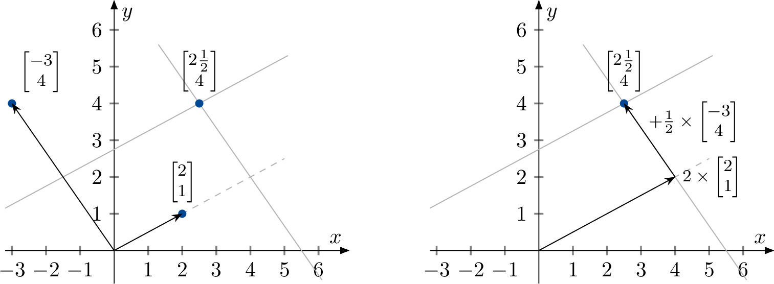
Figure 8.3: The geometrical equivalent of solving a system of equations using the column vector perspective. To construct the solution, draw help-lines through the target point parallel to the vectors and, if necessary, trough the vectors intersecting the parallel help-lines (left figure). Then draw the target point as the sum of these vectors each multiplied by a scalar (right figure).

From the figure, we see that we need two times the vector $\bigl[\begin{smallmatrix}2\\1\end{smallmatrix}\bigr]$ ($x=2$), and half the vector $\bigl[\begin{smallmatrix*}[r]-3\\4\end{smallmatrix*}\bigr]$ ($y=\tfrac{1}{2}$), to reach the target point:

\[ \begin{bmatrix} 2 \\ 1 \end{bmatrix} \times 2 + \begin{bmatrix} -3\\ 4 \end{bmatrix} \times \tfrac{1}{2} = \begin{bmatrix} 4 \\ 2 \end{bmatrix} + \begin{bmatrix} -1 \tfrac{1}{2}\\ 2 \end{bmatrix} = \begin{bmatrix} 2\tfrac{1}{2} \\ 4 \end{bmatrix} \]

8.3 Exercises

Multiplying a vector by a matrix

Exercise 14.

Calculate the following matrix multiplication \[ \begin{bmatrix} 4 & 0 & 1 \\ 0 & 1 & 0 \\ 4 & 0 & 1 \end{bmatrix} \begin{bmatrix} 3 \\ 4 \\ 5 \end{bmatrix} \]

Exercise 15.

Calculate the following matrix multiplication \[ \begin{bmatrix} 1 & 0 & 0 \\ 0 & 1 & 0 \\ 0 & 0 & 1 \end{bmatrix} \begin{bmatrix} 5 \\ -2 \\ 3 \end{bmatrix} \] A square matrix, like the one above, which has only $1$’s on the diagonal and $0$’s everywhere else is called an identity matrix. Any idea why?

Exercise 16.

Calculate the following matrix multiplication \[ \begin{bmatrix} 2 & 0 \\ 1 & 3 \end{bmatrix} \begin{bmatrix} 1 \\ 1 \end{bmatrix} \] Draw the column vectors $\bigl(\begin{smallmatrix}2\\1\end{smallmatrix}\bigr)$ and $\bigl(\begin{smallmatrix}0\\3\end{smallmatrix}\bigr)$. Multiplying by $\bigl(\begin{smallmatrix}1\\1\end{smallmatrix}\bigr)$ just adds the two vectors (do it graphically).

Dual representation

Exercise 17.

Solve this system of equations graphically for $x$ and $y$ from an equation perspective. Write it in column-vector format and solve it graphically from that perspective too. \[ \begin{alignedat}{3} 2x & {}-{} & y &= 1\\ x & {}+{} & y &= 5 \end{alignedat} \]

Exercise 18.

Solve the following systems of equations graphically for $x$ and $y$ from an equation perspective. Write it in column-vector format and solve it graphically from that perspective too.

a. \[ \begin{alignedat}{3} x & {}+{} & 2 y &= 0 \\ 2 x & {}-{} & 4 y &= 8 \end{alignedat} \]

b. \[ \begin{alignedat}{3} - x & {}+{} & y &= 1 \\ \frac{1}{2} x & {}-{} & 2 y &= 1 \end{alignedat} \]

c. \[ \begin{alignedat}{3} x & {}-{} & 2 y &= 3 \\ 2 x & {}-{} & 5 y &= 1 \end{alignedat} \]

d. \[ \begin{alignedat}{3} 4 x & & &= 2 \\ & & y &= 4 \end{alignedat} \]

Exercise 19.

The following set of equations is an example of a system with more equations than variables. \[ \begin{align*} x + 2 y & = 2 \\ x - y & = 2 \\ y & = 1 \end{align*} \]

a. Draw the lines in two-dimensional space that represent these three equations

b. Does a single solution to this system of equations exist?

c. What if the right-hand side of each of the three equations equals $0$?

d. Write the system of equations in the form of a linear combination of two column vectors

e. Is there any non-zero choice of right-hand sides that allows the three lines to intersect at the same point?

Pivots

Exercise 20.

Give three numbers $c$ for which the following matrix does not have three pivots. Explain your answer \[ \begin{bmatrix} 2 & c & c \\ c & c & c \\ 8 & 7 & c \end{bmatrix} \]

Exercise 21.

Give three numbers $c$ for which the following matrix does not have three pivots. Explain your answer \[ \begin{bmatrix} c & c & c \\ 5 & c & c \\ 1 & c & 3 \end{bmatrix} \]

2 \ 1 \end{bmatrix} + \[\begin{bmatrix} -3\\ 4 \end{bmatrix}\] = \[\begin{bmatrix} 4 \\ 2 \end{bmatrix}\]

\[\begin{bmatrix} -1 \tfrac{1}{2}\\ 2 \end{bmatrix}\] = \[\begin{bmatrix} 4 - 1 \tfrac{1}{2} \\ 2 + 2 \end{bmatrix}\] = \[\begin{bmatrix} 2\tfrac{1}{2} \\ 4 \end{bmatrix}\] $$

8.4 Exercises