2 Functions

This chapter is about a number of basic concepts. We will discuss a few functions that you will often encounter, and discuss the concept of limit.

2.1 Functions

Figure 2.1: This relation is a function.

In biology we study the way in which living organisms function, and we look for relations between variables. For example between body size and time, temperature and metabolism, numbers of owls and mice. Figure 2.1 and Figure 2.2 show two such relations. Figure 2.1 concerns the oxygen supply of tissues by hemoglobine (Hb). The amount of oxygen transported by Hb depends on the $\ce{O2}$ concentration in the air. The graph shows the relation between the amount of $\ce{O2}$ bound to Hb and the $\ce{O2}$ concentration in the air in the lung. Figure 2.2 concerns the numbers of owl and mice in a certain area. There is a relation: high numbers of mice let the number of owls increase, but conversely many owls let the number of mice decrease. These processes result in the observed relation.

Figure 2.2: This relation is not a function. The arrows indicate how numbers of owls and mice develop over time. Hence, there is an owl-mice cycle.

Mathematically, a relation between two variables is represented by a function. This is, however not always possible. The mathematical definition of a function $y = f(x)$ requires that the relation is unambiguous, i.e. that for every abscissa-value $x$ there exists only one ordinate-value $y$. In Figure 2.1 this is the case, but not in Figure 2.2. Hence, functions are relations with the special property of unambiguity.

In general mathematical terminology there is a relation between the entities. Functions are a special kind of relation having the property of unambiguity. Figure 2.1 and Figure 2.2 are both relations, but Figure 2.1 is a function, and Figure 2.2 is not. A more abstract definition of a relation is formulated in terms of Set theory¹. The two entities are then represented by sets $X$ and $Y$, and a relation is a set $F$ of ordered pairs or 2-tuples:

\[ F = \{(x,y)\} \text{ where } x \in X \text{ and } y \in Y \]

This is shown in Figure 2.3. So, the relation between $X$ and $Y$ is the set $F$. Very often we are interested in relations between sets containing an infinite number of elements, for example where $X$ and $Y$ are (infinite subsets of) the set of real numbers $\mathbb{R}$. It is then, by definition, impossible to define the relation or function by listing all ordered pairs $(x,y)$. However, the relation can be defined by a function description, which is a recipe to calculate the element $y$ of $Y$ when the element $x$ of $X$ is known.

Figure 2.3: Relations between two sets $X$, and $Y$. On the left, the relation is a function and is represented by the set of ordered pairs $F={(1,C),(2,D),(3,D)}$. The set $X$ is called the *domain* of the function, set $Y$ the *co-domain* and the subset (in gray) of $Y$ consisting of all elements that are mapped from the domain, is called the *image* of $X$ in $Y$. On the right the relation is not a function, for two reasons: one of the elements ($4$) of the domain is not mapped (its mapping is undefined) and the element $3$ maps onto two different elements ($C$ as well as $D$) in the co-domain. Hence, the relation is not unambiguous.

Example 2.1

The function $f$ is characterized by the function description $f(x) = \sqrt{x}$ and has as its domain the set $\mathbb{R}^+$ of positive real numbers, including 0. It’s image is the set $\mathbb{R}^+$.
The function $g$ is characterized by the function description $g(x) = x^2 + 1$. If it has as its domain the set $\mathbb{R}$ then its image is the subset $\{x|x \geq 1 \wedge x \in \mathbb{R}\}$. If its domain is the set $\mathbb{N}$ of natural numbers, then its image is a subset of $\mathbb{N}$.

There are different ways to symbolize function descriptions:

$f(x) = x^2 + 3$
$f:x \rightarrow x^2 + 3$
$f:x \rightarrow y \text{, defined by} \; y = x^2 + 3$
$x \xrightarrow{f} x^2 + 3$

Strictly speaking, you should always give the domain with a function. If the domain is obvious (the set of real numbers $\mathbb{R}$, or in many applications $\mathbb{R}^+$) you can leave it out of the definition. If it is unusual, for example $2 < x < 5$, then you must indicate the domain with the function definition.

In case of composite functions (functions of functions) the third way of symbolizing is often used. For example, the functions

\[ f:x \rightarrow x^2 + 3 \qquad \text{ and } \qquad g:x \rightarrow \sin x \]

can be chained as follows

\[ x \xrightarrow{f} y \xrightarrow{g} z \]

The overall result $h(x)$ is also written as

\[ h = g \circ f \tag{2.1}\]

The meaning of these two notations is that the image $h(x)$ of $x$ is obtained by first applying the function rule $f$ to $x$ and by then applying the function rule of $g$ to the result of $f$. Specifically, this rule is obtained by substituting $y = x^2 + 3$ in $z = \sin y$. This is also often expressed as

\[ z = g(f(x)) = \sin(x^2 + 3) \] In biology some functions are observed more often than others. Below we show these functions in their simplest form. Later we discuss variants of these.

\[ \begin{align*} & \text{straight line:} & f(x) & = x \\ & \text{parabola:} & f(x) & = x^2 \\ & \text{$e$-power:} & f(x) & = e^x \\ & \text{hyperbola:} & f(x) & = \frac{1}{x} \\ & \text{sine:} & f(x) & = \sin x \end{align*} \]

These are displayed in Figure 2.4.

Shifting, stretching, and mirroring of functions

Variants of these functions may be obtained by a number of geometric operations:

stretching or compressing
shifting
mirroring

A fourth operation, rotation, is less relevant for our applications. It is also a more complicated operation. To every operation belongs a rule that is applied to the original function $f(x)$.

\[ \begin{align*} & \text{stretching horizontally by a factor }\alpha & (f \circ g)(x) \text{ where } g(x)=\frac{x}{\alpha} \\ & \text{stretching vertically by a factor }\alpha & (g \circ f)(x) \text{ where } g(x)=\alpha x \\ & \text{shifting by } a \text{ to the right} & (f \circ g)(x) \text{ where } g(x)=x-a \\ & \text{shifting by } a \text{ upwards} & (g \circ f)(x) \text{ where } g(x)=x+a \\ & \text{mirroring over the horizontal axis} & (g \circ f)(x) \text{ where } g(x)=-x \\ & \text{mirroring over the vertical axis} & (f \circ g)(x) \text{ where } g(x)=-x \\ \end{align*} \]

Example 2.2 Two examples.

Shifting 3 to the right: replace every occurrence of $x$ by $x - 3$ (not $x + 3$) in the original function.
Mirroring about the vertical axis (putting the graph upside-down): put a minus sign in front of the original function.

An overview of transformations is given in Figure 2.5.

Figure 2.5: Variants of a function: shifting, mirroring and stretching. The original function is shown in the center graph.

By combining these operations many variants of the original functions can be obtained.

Example 2.3 What will the function $f(s) = \sin{x}$ look like when you

stretch it horizontally by a factor $30/2\pi{}$
then stretch it vertically by a factor $2$
then shift it by $2$ upwards

Sequentially applying these transformations to the original function yields subsequently

\[ \sin{\frac{2\pi}{30}x}, 2\sin{\frac{2\pi}{30}x}, \text{ and finally } 2 + 2\sin{\frac{2\pi}{30}x} \]

$e$-powers

Many processes (functions of time) can be described as $e$-powers. Later on we will see what the origin of this fact is. Except for the basic form $e^t$ (exponential growth) you will see other variants, a few of which are illustrated in Figure 2.6}.

The decreasing $e$-power $F(t)=e^{-at}$ can be encountered with washing out of drugs, dying populations, radioactive decay and other situations. Graphically, you can obtain it by mirroring the basic function $e^t$ on the horizontal axis: replace $t$ by $-t$ (letting time run backwards), and compress time by a factor $a$. $F(t)$ approaches $0$ asymptotically.

The function $G(t) = 1 - e^{-at}$ ($F$ upside-down and raised) is a function that is often encountered in exchange processes: a temperature slowly adapting to the tmpereature outside, leveling of concentration differences on the in- and outsides of the cells. In this example, $G(t)$ approaches $1$ asymptotically.

The function $H(t) = e^{-at} - e^{-bt}$, the difference between two decreasing $e$-powers, has a completely different shape. The function starts at $0$, increases (if $b > a$) to a maximum, and then slowly decreases to $0$. Such functions are often the result as a result of composite processes, for example a hormone entering and leaving an organ.

Half-life and doubling time

The rate at which the decreasing $e$-power approaches $0$ is determined by the parameter $a$: the function decreases faster with large than with small values of $a$. Rather than referring to $a$ directly, another way of characterizing this rate is the half-life, the time that it takes the process to reach half of the original value. In principle, you could determine the time that it takes to reach half the original value. Starting, for example with EUR 1800 on a bank account, and taking EUR 100 from it every month, it takes 9 months to reach half the original value. However, starting at EUR 1000, it takes 5 months at the same rate. At every point in time, the half-life of this process is different, and hence, you cannot speak of the half-life of this process. However, with the decreasing $e$-power you can.

Example 2.4 Take the function $F(t) = 100 e^{-0.4t}$, which decreases from 100 to 0. How long does it take to reach the value 50? Let that be $T$ time units. Then it should be true that $F(T)=50$ or, $100e^{-0.4T} = 50$. This gives $e^{-0.4T} = 1/2$. Take the natural logarithm of both sides: $-0.4T = \ln{1/2} = -\ln{2}$. Rearrange: $T = \frac{\ln{2}}{0.4} \approx 1.75$.

That was the half-life when starting from a value 100 on $t = 0$. What would the half-life be when starting from a different point in time? Take a random time point $t=a$. Then $F(t) = e^{-0.4a}$. $T$ time units later (on $a+T$) the function should have half the value compared to time point $a$:

\[ \begin{align*} F(a+T) & = \frac{1}{2} F(a) \\ 100 e^{-0.4(a + T)} & = \frac{1}{2} 100 e^{-0.4 a} & \text{applying the function }F \\ e^{-0.4 T} & = \frac{1}{2} & \text{simplifying} \end{align*} \]

It is the same expression that we obtained before, also with the result $T = \frac{\ln{2}}{0.4}$. Apparently, starting from any point in time we arrive at the same value for $T$, and therefore, we can speak of the half-life of this process.

The example can be easily generalized. Any decreasing $e$-power has a half-life $T_{1/2}$ with the following value:

Remark 2.1. For $F(t) = C e^{-at}$ the half-life $T_{1/2}$ equals $T_{1/2} = \frac{\ln{2}}{a}$

Similarly, for increasing $e$-powers we can calculate a doubling time $T_2$ as follows:

Remark 2.2. For an increasing $e$-power, the doubling time $T_2$ equals $T_2 = \frac{\ln{2}}{a}$

Apart from $e$-powers would there be any other functions for which a constant half-life or doubling time can be defined? It can be shown mathematically that this is not the case. Therefore it is not very useful to speak of the half-life or doubling time in case of any other function.

Hyperbolas and enzyme reactions

Almost all compounds in living cells are made by enzymes, every compound being the product of a specific enzyme. The rate at which these enzymes work is of utmost importance to the vital function of the cell. There are fast and slow enzymes, and the temperature is an important determining factor for the rate. But the rate also depends on the concentration of the enzyme substrate (the compound that is converted by the enzyme). They are related almost obviously by a function that increases with the substrate concentration, but what does it look like exactly?

Simply stated, when doubling the substrate concentration $S$, an enzyme molecule will encounter a substrate molecule twice as often, and you expect that its production rate, $V$, will also double. But that is true only for low values of $S$. For each substrate molecule that it turns over to a product molecule the enzyme needs a certain amount of time. During this time its binding site is occupied and it cannot bind a substrate molecule, even if it encounters one. At very high substrate concentration, the enzyme is presented with a substrate molecule as soon as it has finished making a product molecule, and it will have reached the upper limit of its turnover time. The theory (a classic from 1913 by Michaelis and Menten, will be discussed later) tells us the shape of this relation between $S$ and $V$. It is given by

\[ V = \frac{a S}{b + S} \]

This function is —perhaps not immediately recognizable— a hyperbola. It can be obtained from the basic function ($1/x$) by putting it upside-down and then shifting it so that it passes through the origin. As with every hyperbola, it also has a second `branch’ that lies entirely in the negative $S$ domain. This part has no physical meaning or interpretation.

Interpretation of $a$ and $b$

The two parameters of the function, $a$ and $b$, both have clear physical interpretations, and can also be readily deduced from the graph.

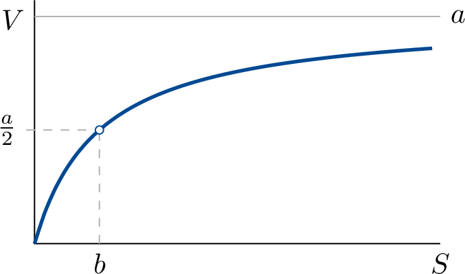
Figure 2.7: Rate of an enzyme reaction. Interpretation of the parameters $a$ and $b$.

The parameter $a$ determines the upper bound of $V$, which is the limit value that $V$ approaches when $S$ becomes very large. From the function equation this is not immediately clear, because both numerator and denominator become very large. It helps to rewrite the function (divide numerator and denominator by $S$):

\[ V = \frac{aS}{b+S} = \frac{a}{\displaystyle \frac{b}{S} + 1} \]

For very large values of $S$, the term $\frac{b}{S}$ tends to $0$, and $V$ tends to the value $a$. The interpretation of the parameter $b$ is obtained as follows. When the substrate concentration equals the value $b$, then $V$ will equal the value $1/2 \,a$ (just fill in). In other words: $b$ equals the substrate concentration at which the enzyme reaches half the maximal rate. In enzyme kinetics, $a$ and $b$ get their own symbols, namely $V_\text{max}$ en $K_\text{M}$. $K_\text{M}$ is also called the Michaelis constant.

In other disciplines of biology (ecology, microbiology) the same hyperbolic function can be found, often with their own symbols for the parameters $a$ and $b$.

“Frankenstein functions”, Min and Max

Often practical applications can not be described by a single neat mathematical formula, but has to be glued together from parts of different functions.

Example 2.5

A vessel of 500 liter is filled at a rate of 2 liter per minute. Once it is filled, it will overflow, so that the content does not increase anymore. Hence, $Q(t)$, the content of the vessel, increases linearly until the moment it starts to overflow, and then runs horizontally. This gives a broken, Frankenstein-like function description:

\[ Q(t) = \begin{cases} 2t & \text{for} \quad t \leq 250, \\ 500 & \text{for} \quad t > 250 \end{cases} \]

for which first the time point until overflow, $t=250$ has to be calculated.

There is another, often simpler way of describing the function by using the functions Min and Max. The graph consists of fragments of the two functions $y=2t$ and $y=500$. If you draw both entirely, then at any point in time $t$, $Q(t)$ is equal to either of the two. Which one? That’s simple: the one with the lowest value. This yields a recipe for $Q(t)$ different from the previous one:

\[ Q(t) = \text{Min}(2t,500) \]

It will be clear how the function Min is defined: for any time point $t$ it takes the smallest value of the expression between brackets (there could be more than two expressions between the brackets). The equivalent holds for the function Max.

Note that when writing the function this way, you do not have to calculate the intersection point (in this case, $t=250$ it was easy, often it is not.) For this reason and because of the compact notation, the functions Min and Max are handy. They are available in many computer programs (Also in Excel, for example).

2.2 Limits

In the previous section the concept of limit was touched upon. In mathematics this is a central concept. As an average user you do not have to know its nitty gritty details, but since you will encounter it regularly you have to know something about it.

When you substitute the value $x=2$ in the function equation $f(x) = x^2 + 3$, you will find $f(2) = 7$. With some functions, such substitutions will yield a problem for certain values of $x$. Two situations will occur often:

The function is a quotient, and for particular values of $x$ numerator and denominator become 0. For example, $f(x) = \frac{\sin x}{x}$. For $x = 0$ the function is not defined. At the same time you will see that for small values of $x$ (where the function is perfectly defined), the value of the function approaches 1: you can approach 1 ever closer by decreasing $x$ closer to 0. We then say:\[\lim_{x \to 0} \frac{\sin x}{x} = 1\] Pronounced as: “the limit for $x$ approaching 0, of $\frac{\sin x}{x}$ equals 1”.
Asymptotes: you want to say something about the value that a function approaches when $x$ becomes very large. However, `very large’ is not a number. For example: $g(x) = e^{-x}$. The value of the function clearly approaches 0 but there is no value of $x$ for which it is ever equal to 0. We then say: \[\lim_{x \to \infty} e^{-x} = 0\] Pronounced as: “the limit, for $x$ approaching infinity, of $e^{-x}$ equals 0”.

We discuss these two cases in more detail.

Limits of quotients

The first case: quotients. The previous example was a bit far-fetched. But the same happens with derivatives, actually with all derivatives. The concept of derivative is defined as a limit. You know the story: if you want to know the slope of a function in a particular point $x$, then you take another point a bit further away ($x+h$) and divide the increase by the difference $h$, and then you decrease the difference $h$ until the second point coincides with the first point. However, as soon as these points coincide, the quotient becomes an undefined $0/0$. That’s why the derivative is defined as a limit. An example:

We determine the derivative of $f(x) = x^2 + 1$ in the point $x = 3$. The function there has a value $f(3)=10$ (the graph has been re-scaled somewhat). Take a point little further away, $x = 3 + h$. Determine the value of the function there, and divide the growth of $f(x)$ by the difference in the $x$ coordinate. You get the slope over the interval $[3, 3 + h]$:

\[ \frac{f(3+h) - f(3)}{h} = \frac{\left[ {(3+h)}^2 + 1 \right] - \left[ 3^2 + 1 \right]}{h} \]

which yields:

\[ \frac{6h + h^2}{h} \]

The result is not the desired slope in $x = 3$, but an average slope over the interval (with this function that has an increasing slope this average slope is higher than the desired slope). The smaller $h$, the better; but you cannot just substitute 0 for $h$ because this would yield $0/0$ which is not defined. Therefore, you take a more careful approach in which you follow what happens to the slope as the second point approaches $x = 3$; $x = 3$ itself is not considered. Under this condition (which means that $h \neq 0$) you can say: $\frac{6h + h^2}{h}= 6 + h$, and this approaches 6 as $h$ decreases. We now say:

\[ \lim_{h \to 0} \frac{6h + h^2}{h} = 6 \] This means: by letting $h$ approach $0$ close enough, you can let the value of the quotient approach 6 as close as you want.

More general, you get the following definition:

Definition 2.1 (Derivative of a function) The derivative $f'(x)$ of a function $f(x)$ equals \[ f'(x) = \lim_{h \to 0} \frac{f(x+h) - f(x)}{h} \]

Calculating such a limit may not always be successful. Sometimes the quotient increases more and more as $h$ approaches 0, and other complications may also arise. Or, with limits you have to take care: they are not always defined. Also with derivatives this may happen. In that case a function (in a certain point) just does not have a derivative. We then say that the function is not differentiable in that point. In Chapter 3 we will return to this.

Asymptotes

The second case: asymptotes. Many functions (straight lines, parabolas, $e$-powers) increase indefinitely, and can reach any value if you continue long enough (decreasing is also a possibility, of course). But there exist also functions the slowly tend to a ‘boundary value’ that they approach closer and closer, but never actually reach (the word ‘asymptote’ originates from the Greek and means ‘not coincide’). Such functions are found a lot in biology. We already gave an example: $f(x) = e^{-x}$, which tends to 0 for large $x$. We already mentioned the way of formulating:

\[ \lim_{x \to \infty} e^{-x} = 0 \]

The meaning of this is: by taking a large enough value of $x$ you can get the value of the function arbitrarily close to 0.

Big-$O$ notation

The big-$O$ notation, $O(f(x))$, is often used to characterize the behaviour of a function $f(x)$ when $x$ tends to infinity. The expression $O(f(x))$ is called the order of the function $f(x)$. A (informal) definition of the statement “$O(f(x))$ is $g(x)$”, is that there must be a number $x_0$ and a positive constant $M$ such that $|f(x)| \leq M g(x)$ for all $x > x_0$. A requirement of $g(x)$ is that it must be a strictly positive function for ($x > x_0$). The trick is to use simple functions $g(x)$ to characterize the behaviour of potentially complex functions $f(x)$.

Example 2.6 (Memory used by an algorithm) An algorithm uses an amount of memory equal to $m(n) = 5 n + 4 n^2 + n^3$ when the input is a $n \times n$ matrix. We can then state that $O(m(n))$ is $n^3$.

Proof. We have to prove $5 n + 4 n^2 + n^3 < M n^3$ for some value of M and all $n > n_0$. Let’s take $M = 2$. We find $n_0$ by solving $5 n + 4 n^2 + n^3 = 2 n^3$:

\[ \begin{align*} 5n_0 + 4 n_0^2 + n_0^3 &= 2 n_0^3 \\ 5n_0 + 4 n_0^2 - n_0^3 &= 0\\ 5 + 4 n_0 - n_0^2 &= 0 \\ n_0 &= 5 \end{align*} \]

So, this is true for all values of $n > 5$.

The reason that such knowledge is useful is that it allows you to compare the resource usage of alternative algorithms when the size of the problem becomes very large. Algorithms of lower order are then preferred to those of higher order.

We can establish a sequence of orders for the following simple functions, where the order increases from top to bottom:

\[ \begin{align*} & K \; \text{(constant)} \\ & \log_{b}(n) \\ & n \\ & n \log_{b}(n) \\ & n^2 \\ & n^p \; \text{for increasing powers } p \\ & 2^n \\ & 3^n \\ & k^n \; \text{for increasing bases } k \\ & n! \\ & n^n \end{align*} \]

It is handy to keep this sequence in mind because in general a function $f(n)$ is $O(g(n))$ where $g(n)$ is the dominant term in $f(n)$. And the dominant term in a function is the one with the hihghest order in the list above.

Infinity

This needs some explanation. What does that actually mean, infinity? Is it a real number? If so, can we calculate with it, just like the numbers that we already know? If not, does it fall in the domain of the function (and what are we talking about then)?

Answer: no, there is no real number called infinity or $\infty{}$.
Question: what does it mean then?
Answer: the symbol $\infty{}$ is not the name of a mathematical object; it only occurs as part of expressions in combination with the symbols $\to{}$ and $\lim{}$. This combination must be properly defined, and as we saw above, it is: “by choosing $x$ large enough $\dots$” (the mathematical definition is more precise but boils down to this in essence).

The expression “$\lim_{x \to \infty}$” therefore has a very concrete meaning, in which no mystical stories about infinity appear. The individual symbol $\infty{}$ has no meaning at all, and you cannot use it as such. Expressions like

\[ \frac{7}{0}=\infty \quad \text{and} \quad \lim_{x \to \infty} \left( x^2 + 3 x \right) = \infty \]

have no meaning and are plain wrong! You should then say that the quotient and the limit are not defined, or do not exist.

2.3 Exercises

Sketch these functions

Exercise 1.

$y = - e^x$

Exercise 2.

$y=-\ln x$

Exercise 3.

$y = 2^{x-3}$

Exercise 4.

$g(x) = |x-2|$

Analyze these functions

Exercise 5.

$f(x) = \dfrac{x+1}{x-2}$

Exercise 6.

$f(x) = x \cdot \ln(x)$ for $x > 0$

Exercise 7.

Consider $f(x) = - 4x^2 + 4x +24$

a. Solve $f(x)=0$ for $x$.

b. Give the derivative $f'(x)$

c. Sketch the graph of $f(x)$. Please indicate any minima, maxima and intersections with the x- and y-axes.

Limits

Exercise 8.

$\lim_{x \to 3} \dfrac{x^2 - 2x - 3}{x^2 - 9}$

Exercise 9.

$\lim_{x \to \infty} \dfrac{ax}{b + x}$

Exercise 10.

$\lim_{x \to \infty} \dfrac{ax}{b^2 + x^2}$

Applications

Exercise 11.

The concentration of intravenous medication in the blood as a function of time is given by:

\[ y(t) = a (e^{-bt}-e^{-ct}), \quad c > b > 0 \quad \mathrm{and} \quad a > 0 \]

a. Show that $y(t) > 0$ for $t > 0$

b. Find the maximum of $y$ and at which time $t$ this is reached

c. Find the time $t$ where the graph has a inflection point

d. Sketch the graph for $t > 0$ for $a = c = 2$ and $b = 1$

Exercise 12. Time complexity of algorithms

Time complexity measures the computational effort required by an algorithm based on the size of its input. You are given two sequence alignment algorithms: Algorithm A, which has a polynomial time complexity, and Algorithm B, which has a linear time complexity. Their respective time complexities are:

Algorithm A: $T_A(n) = n^2$
Algorithm B: $T_B(n) = 50 n$

where $n$ is the length of the sequences being aligned.

a. Sketch the time complexity functions of the two algorithms for sequence lengths $n$ ranging from 0 to 100.

b. Calculate processing times for the following specific sequence lengths:

Determine which algorithm is faster when aligning two sequences of length 30.
Determine which algorithm is faster when aligning two sequences of length 80.

c. Determine the sequence length $n$ at which the two algorithms take the same amount of time.

d. What is the order $O(T_A(n))$ and $O(T_B(n))$ of both algorithms?

Exercise 13. Comparing efficiency of two algorithms

The number of calculations performed in two algorithms A1 and A2 solving the same problem of size $n$ (discrete values) are:

Algorithm A1: $C_1(n) = n + 1.2 n^2$
Algorithm A2: $C_2(n) = n + 3 n \log(n)$

What are the orders of these two functions and which one is more efficient (uses less calculations) for large values of $n$?

Exercise 14. Activation functions for neural networks

Activation functions play an important role in artificial neural networks. They function as thresholds converting a gradually changing input signal to a “decision”. Below are a few examples.

a. Describe the domains and ranges or images of each of the following activation functions and also draw graphs of them

The Heaviside or step function: \[ \mathcal{H}(x) = \begin{cases} x < 0 & 0 \\ x \geq 0 & 1 \end{cases} \]
The logistic function: \[ \phi(x) = \frac{1}{1 + e^{-x}} \]
The rectifier linear unit (ReLU) function (This is the function most used in deep neural networks) \[ R(x) = \text{max}(0,x) \]
A variant of the previous function is the the “leaky ReLU”: \[ LR(x) = \text{max}(0.1 x, x) \]

When optimizing a neural network, during the “learning phase”, the derivative of the activation function is needed in most learning algorithms to calculate updated signal weights in the neural network. Weights are adapted proportional to the derivative of the activation function.

b. Write down the formula’s of the derivatives of each of the activation functions above and sketch their graphs. What could be a disadvantage of the Heaviside function in learning algorithms? And of the logistic function?

The entire fundament of mathematics can be formulated in terms of Set theory, which is why this may be called a fundamental definition.↩︎