3 Differentiation

Differentiation is one of the basic skills of every scientist. You will encounter it when thinking about processes (changing conditions in time), and it is also part of a variety of techniques, such as finding a maximum or minimum, drawing a curve through data points, and approximating a difficult function by a more convenient one. In this chapter we discuss some of the material from high school, and expand the concept of derivative to a function of two or more variables. Subsequently, a number of techniques will be discussed: search for extremes, curve fitting, and locally linearize.

3.1 The derivative

Definition

Definition 3.1 (Derivative of a function) The derivative of a function $f$ in the point $x$ is defined as the limit \[ f'(x) = \lim_{h \to 0} \frac{f(x+h) - f(x)}{h} \]

The geometrical interpretation of the derivative $f'(a)$ is the slope of the tangent of $f(x)$ at the point $x=a$. If $f$ is a function of time, then $f'(t)$ gives the rate of change of $f$ at time $t$.

The derivative is defined as a limit and as we saw in Chapter 2 it may happen that a limit is not defined (does not exist). If it does exist at a particular point, then the function is called differentiable at that point; differentiability is a property that applies to a given point, but for the same function may not apply at another point. When we say (without mentioning in which point) that a function is differentiable, we mean that it is differentiable everywhere.

Notation

As you know, the derivative $f'(x)$ is also written as $\dd{f}{x}$. The notation $f'(x)$ is due to the Italian mathematician Joseph Louis Lagrange (born Giuseppe Lodovico Lagrangia). The classical notation $\dd{f}{x}$ is due to Gottfried Wilhelm Leibniz, who, together with Isaac Newton, is one of the inventors of the calculus. The classical notation is somewhat awkward because it looks like a quotient but certainly isn’t one. Yet, we use it very often. When using that notation, it is important to realize that you can not treat $\dd{f}{x}$ as a quotient. You should consider the notation more as a remembrance of the fact that the derivative is the limit of a quotient as given in Definition 3.1.

Differentiability

Differentiability is something you should be aware of in in biological applications. In practice you will encounter a lot of functions that are not differentiable in certain points because they

make a jump
contain a kink
suddenly stop somewhere

(These are the three possibilities). By taking the derivative at each point of $f$ a new function arises from $f$, the derivative function $f':x \rightarrow f'(x)$. This function can in turn be differentiated, in that way generating the second derivative $f''(x)$, etc. Here again, differentiability is of interest: it is quite possible that a function is twice differentiable but not a third time.

The derivative and the function defining the derivative are, strictly speaking, two different matters.

Example 3.1 Take $f:x \rightarrow x^2 + 3$. Then the derivative at $x=4$ is a number: $f'(4)=8$. The function defining the derivative, however, is not a number but the mapping: $f':x \rightarrow 2x$.

In practice, this distinction is usually not made as sharp, and we say “the derivative of $f(x)=x^2 +3$ equals $f'(x)=2x$”. Often this somewhat sloppy terminology is of no consequence. Sometimes it is necessary to make the distinction.

Differentiation from first principles

The definition of the derivative (Definition 3.1) allows a derivation of a function $f'(x)$ describing the derivative for a given mapping $f(x)$, by just applying it.

Example 3.2 We want to have a function describing the derivative of the function $f(x) = x^2 + x -1$ in all admissible points $x$. We can apply the definition: \[ \begin{align*} f'(x) & \equiv \lim_{h \to 0} \frac{f(x+h) - f(x)}{h} \\ & = \lim_{h \to 0} \frac{{(x + h)}^2 + (x + h) - 1 - (x^2 + x - 1)}{h} \\ & = \lim_{h \to 0} \frac{x^2 +2xh + h^2 + x + h - 1 - x^2 - x + 1}{h} \\ & = \lim_{h \to 0} \frac{2xh + h^2 + h}{h} \\ & = \lim_{h \to 0} 2x + h + 1 \\ &= 2x + 1 \end{align*} \]

This is what we call differentiation from first principles. Clearly this becomes a lot of work if you have complicated expressions. The example demonstrates, however, that the definition is sufficient for deriving a function description for $f'(x)$.

Another example concerns the exponential functions like $f(x) = a^x$. This teaches us something about the origin of Euler’s number:

Example 3.3 (The origin of Euler’s number) Applying the definition of derivative to $f(x) = a^x$ yields: \[ f'(x) = \lim_{h \to 0} \frac{a^{x+h} - a^{x}}{h} = \lim_{h \to 0} \frac{a^{x} a^{h} - a^{x}}{h} = a^x \lim_{h \to 0} \frac{a^{h} - 1}{h} \] This shows that the derivative of $a^x$ is the function itself times the limit $\lim_{h \to 0} \frac{a^{h} - 1}{h}$. This limit is independent of $x$, and therefore, if it exists, is a constant number that depends only on the value $a$. When we approximate this limit for a few values of $a$ by choosing a tiny value of $h$ we observe something peculiar:

a	limit
2	0.6932
3	1.0986
4	1.3863
8	2.0794

First notice that every time as $a$ doubles from 2 to 4 to 8, a value 0.6932 is added to the limit, and second, the series suggests that there is a number, let’s call it $e$, between 2 and 3 for which the limit equals 1. Hence, for this number $e$ the derivative of $e^x$ is equal to itself! If we had not known about this number, this is a way we could have found out that it exists.

Differentiation using a limited set of rules

As you know, there are mathematical rules which make it possible to express the derivative of a composite function in those of the constituent functions. As a result, it is possible to calculate in a large number of derivatives from a set of basic derivatives without having to rely on the definition of the derivative. The basic functions are the following:

A list of common derivatives

\[ \begin{align*} f(x) & = c & f'(x) & = 0 \\ f(x) & = x^r & f'(x) & = rx^{r-1} \\ f(x) & = \ln{x} & f'(x) & = x^{-1} \\ f(x) & = e^x & f'(x) & = e^x \\ f(x) & = \sin{x} & f'(x) & = \cos{x} \\ f(x) & = \cos{x} & f'(x) & = -\sin{x} \\ \end{align*} \]

And here are the most important rules for differentiation of composite functions:

Rule for differentiation

Constant rule: \[h(x)=cf(x) \qquad h'(x) = cf'(x)\]
Summation rule: \[h(x) = f(x) + g(x) \qquad h'(x) = f'(x) + g'(x)\]
Product rule: \[h(x) = f(x) \cdot g(x) \qquad h'(x) = f'(x) \cdot g(x) + f(x) \cdot g'(x)\]
Quotient rule: \[h(x) = \frac{f(x)}{g(x)} \qquad h'(x) = \frac{f'(x) \cdot g(x) - f(x) \cdot g'(x)}{{\left( g(x) \right)}^2}\]
Chain rule: \[h(x) = (f \circ g)(x) \qquad h'(x) = (f' \circ g)(x) \cdot g'(x)\]

Notes about the Chain rule

In the formulation of this rule we have used the “$\circ{}$” notation for function composition, as introduced in Equation 2.1. This is a somewhat tedious but also very useful rule, because it simplifies the differentiation of complex functions. In Leibniz notation the rule is often easier to remember, because the variable with respect to which differentiation takes place is explicitly indicated:

\[ \dd{f}{x} = \dd{f}{g} \cdot \dd{g}{x} \]

And it is also often written in Lagrange notation as:

\[ f(g(x))' = f'(g(x)) \cdot g'(x) \] In the chain rule we perform a substitution, although this is not always made explicit. In the original function $h(x)$ you replace an expression in $x$ by a variable $g$, so that you obtain a new function $f(g)$ that can be more easily differentiated. An example: in the function definition $\sin{(x^2 + 1)}$ of the function $f$ you replace the expression $x^2 + 1$ by the variable $g$. With this, you define two new functions, namely $g(x)=x^2 + 1$ and $f(g)=\sin{(g)}$¹. The new function, $f(g)=\sin{(g)}$, can be readily differentiated, namely $f'(g)=\cos{(g)}$. Now using the chain rule, and re-substituting $g=x^2 + 1$ we obtain:

\[ h'(x) = f'(g) \cdot g'(x) = \cos{(g)} \cdot 2 x = 2 x \cos{(x^2 + 1)} \]

We give a few examples to demonstrate the use of each rule.

Example 3.4 (The summation rule) \[ \begin{split} f(x) &= 3 x^4 - 12 \sqrt{x} - \frac{5}{x^3} \\ f'(x) &= 3\cdot4 x^3 - 12 \cdot \frac{1}{2} x^{-1/2} - 5 \cdot (-3) \cdot x^{-4} \\ &= 12x^3 - \frac{6}{\sqrt{x}} + \frac{15}{x^4} \end{split} \]

Example 3.5 (The product rule) \[ \begin{split} h(t) &= t^3 \ln t \\ h'(t) &= 3t^2 \ln t + t^3 \frac{1}{t} \\ &= t^2(3 \ln t + 1) \end{split} \]

Example 3.6 (The quotient rule) \[ \begin{split} g(x) &= \frac{e^x -4}{x^2 + 7} \\ g'(x) &= \frac{\left( e^x - 4 \right)' \left( x^2 + 7 \right) - \left( e^x - 4 \right) \left( x^2 + 7 \right)'}{{\left( x^2 + 7 \right)}^2} \\ &= \frac{e^x \left( x^2 + 7 \right) - \left( e^x - 4 \right) 2x}{{\left( x^2 + 7\right)}^2} \\ &= \frac{e^x \left( x^2 - 2x + 7 \right) + 8x}{{\left( x^2 + 7 \right)}^2} \end{split} \]

Example 3.7 (The chain rule) \[ \begin{split} f(x) &= {\left( x^3 + 4x \right)}^5 \\ f'(x) &= 5{\left(x^3 + 4x \right)}^4 \left(3x^2 + 4 \right) \\ \\ r(x) &= \cos{2\pi x} \\ r'(x) &= -\sin{2\pi x} \cdot 2\pi = -2\pi \sin{2\pi x} \end{split} \]

Example 3.8 (A combination of rules) \[ \begin{split} g(t) &= \left(2 t^3 -3\right) e^{-5t^2} \\ g'(t) &= \left( 2t^3 - 3 \right)' \cdot \left( e^{-5t^2} \right) + \left( 2t^3 - 3 \right) \cdot \left( e^{-5t^2} \right)' \\ &= \left( 6 t^2 \right) \cdot \left( e^{-5t^2} \right) + \left( 2t^3 - 3 \right) \cdot \left( e^{-5t^2} \cdot (-10t) \right) \\ &= \left( 30t + 6t^2 - 20t^4 \right) e^{-5t^2} \end{split} \]

3.2 Functions of two variables and their derivatives

Most functions you have come across so far are functions of one variable. But a quantity may depend on two or more other quantities, and the relation is then described by a function of two or more variables. Graphically you can imagine a function that depends on two variables as a mountain region. gives an example: a quantity $z$ that depends on two other quantities $x$ and $y$ according to the function

\[ z = f(x,y) = 2 - 0.5 {(x - 1.25)}^2 - 0.5 {(y-1)}^2 \]

The value of the function in point $P = (1.7, 1.25)$, for example, is

\[ z = f(1.7,1.25) = 2 - 0.5 {(1.7 - 1.25)}^2 - 0.5 {(1.25 - 1)}^2 \approx 1.87 \]

Figure 3.1: A function of two variables and a point $P=(x_0, y_0)$ in the $x$—$y$ plane at which $z_0=f(x_0,y_0)$ is calculated.

Of such functions it is also possible to indicate at what rate they change (graphically: their steepness). It is just a little more complicated. One can not speak of the slope at the point $P$, since the $x$-direction (to the right) the slope is different from the $y$-direction (toward you in the line of vision). The function has therefore two derivatives, called the partial derivatives of $f$: one in the $x$-direction and another in the $y$-direction (see Figure 3.2).

Partial derivatives

To obtain the partial derivative to $x$ you just differentiate the function to $x$, while treating $y$ as a constant. In an analogous manner you obtain the partial derivative to $y$:

\[ \begin{align*} f_x(x,y) & = -(x - 1.25) \\ f_y(x,y) & = -(y - 1) \end{align*} \]

The index below $f$ indicates to which of the variables the original function was differentiated. The notation $f'$, that is used for functions of a single variable, cannot be applied here.

Example 3.9 In Figure 3.2} you see the point $P = (x_0, y_0) = (1.7, 1.25)$. Calculate both partial derivatives in $P$:

\[ f_x(P) = -(1.7 - 1.25) = -0.45 \; \text{,} \qquad f_y(P) = -(1.25 - 1) = -0.25 \]

Both slopes are negative and this is in accordance with the graph where, in the point $P$, $f$ decreases both in the $x$- and $y$-directions.

Notation

Also for partial derivatives, there is a notation that is equivalent to the Leibniz notation: $f_x(x, y)$ is written as $\pp{f}{x}$ (curved d’s [$\partial$], not to be confused with delta [$\delta{}$]). This notation is used a lot, because it is much more clearly shows the variable with respect to which the function is differentiated. In the Lagrange notation you might sometimes forget to write down the index. This is not possible in the Leibniz notation.

The gradient

For a function of one variable you can display the derivative by plotting $f'(x)$ against $x$. For a function of two variables this is less straightforward, since here two partial derivatives belong to each point $(x,y)$. One can, however, display a property called the gradient, as it is called, in the $(x,y)$ plane, using small arrows. From these arrows you can directly derive the size of the two partial derivatives. In Figure 3.3} you see how the gradient field of the previous example looks like.

From such a gradient field it is possible to read several properties of a function. The length of the arrows indicates the direction and size of the steepest slope of the function at that point. In the previous point $P$ (the one in Figure 3.3) it is the slope in the direction somewhere between west and south-west. If $f$ describes the shape of a mountain, then you can derive from the gradient field how a ball, put down in $P$, would descend (both direction and acceleration). Both direction and size of this steepest slope can be calculated as the vector addition of these from the slopes in the $x$- and $y$-directions.

3.3 Applications of derivatives

Derivatives are widely used in biology. This is hardly avoidable: when studying processes (= variables that change, so: functions of time) also the rate at with which those processes occur (the derivatives of these functions) are of interest. Additionally, there are also some commonly used methods in which derivatives are used. In the next sections, we discuss three such methods:

finding maxima and minima
curve fitting: finding the best-fitting curve with a set of measured values
numerical approximation of (awkward or complicated) functions

Finding extremes

In this section we will discuss the finding of extremes (maxima or minima) of a function. This subject is supposed to have been treated in your preparatory training, so we will only summarize the main results.

To find the extremes of a function $f$ you differentiate the function, and subsequently try to solve the equation $f'(x)=0$ for $x$. Then, you substitute this solution in $f$. By means of this procedure you may find the extremes, however the story is not complete. You can both find too many and too little $x$-values:

Too many: The equation $f'(x)=0$ can have more than one solution, of which only one can be the global minimal or maximal extreme. Moreover, $f'(x)=0$ gives the maxima and minima of the function, and (if they exist) also the horizontal inflection points where the function flattens, but the sign of the slope does not change. So you still have to figure out what the peaks and valleys are. There is a neat way to distinguish maxima, minima and inflection points by considering the sign of the second derivative, but usually it is easier to calculate which of the candidate points yields the largest value of the function. This should be done anyway if the function has several peaks. It could also be that all candidates have to be rejected, if the function increases or decreases indefinitely. In the first case any maxima found are local maxima, and in the second case any minima found are local minima.
Too little: with this method you only find $x$-values in differentiable points of the function. However, an extreme could be present in a point where the function is not differentiable, for example at a kink or a jump, and —especially— at the edges of a domain on which $f$ is defined. Many functions encountered in biology start or end abruptly, and often have a so-called boundary extreme. Figure 3.4 shows two examples of such functions.

Figure 3.4: By only studying the derivative you could miss the true global maximum or minimum. On the right: the function has a kink in the maximum, and is therefore not differentiable at this point.

If you know all parameters (coefficients) of a function, and you can, therefore, draw a graph of it, it is often immediately clear whether it has extremes, and where these are, approximately. If that is not the case, a more systematic analysis of the function is needed.

To summarize:

Finding extremes

Differentiate $f$, calculate all $x$ for which $f'(x)=0$, and calculate the values for $f$ in all these points.
Determine the values of $f$ where the function is not differentiable.
Determine $f$ at the boundaries of its domain(s).
Choose from the previously obtained points the extremes

Clearly, this procedure is only successful if the number of points that it yields is finite.

Extremes of $f(x,y)$

How do you find the extremes of a function of two variables? Actually, in the same way. Only now both partial derivatives should be set equal to zero. This yields two equations, which can be solved for $x$ and $y$. The rest is basically the same: figure out which of the points found is the global extreme, and consider whether there are extremes at the boundaries or at other points where the function is not differentiable.

Example 3.10 We search for the maximum of the function

\[ z = f(x,y) = 1 + 0.8x^2y - 0.5y^2 \] In the maximum both partial derivatives should equal zero:

\[ f_x(x,y) = 0 \quad \text{and} \quad f_y(x,y) = 0 \]

so that

\[ 1.6 xy = 0 \quad \text{and} \quad 0.8 x^2 - y = 0 \]

It is easy to show that there is only one point, the origin $(0,0)$, that satisfies both equations. The value of the maximum there equals $f(0,0)=1$. This is a maximum and it is just a local maximum. The function $f$ does not have a global maximum, because at any fixed value of $y$ we can let $f(x,y)$ increase to extremely high values by increasing $x$.

The “best fitting” curve through measurements

A typical problem of the experimental biologist is the following. You have a set of measurements that you know (suspect, heard, hoping) are an $e$-power (or a straight line, a hyperbole or something else). Which $e$-power is still open. The question now is: how do you find the $e$-power that best suits your measurements? The techniques by which this problem is being addressed are known as parameter estimation or curve fitting.

You performed an experiment with an enzyme. You have measured the rate $v$ at which the substrate is consumed by the enzyme at different substrate concentrations $s$. The purpose of the experiment is to find the relation between $v$ and $s$.

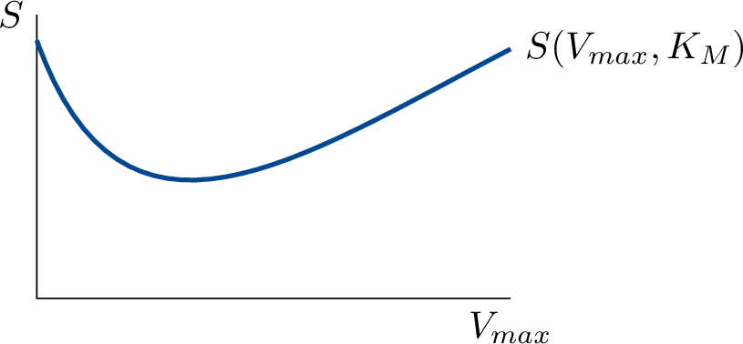
Michaelis-Menten theory tells that it must be a hyperbola: \[ v = \frac{V_\text{max} s}{K_\text{M} + s} \]

But you have to figure out now which hyperbola, or which $V_\text{max}$ and $K_\text{M}$. In the diagram, you see three, apparently none of which is a best-fit. The question is: how do you find the best fitting hyperbola through these points, or the best $V_\text{max}$ and $K_\text{M}$? You will need to be sure that no hyperbola will exactly pass through all the points. Reality —and certainly biological reality— seldom adheres exactly to theory, and even if it did, your measurements will contain errors.

If you want the “best fitting function”, then you should define precisely what you mean by that. What should a measure of fit look like Figure 3.5 shows a function $f$ and five measurements $(x_1,y_1), \ldots, (x_5, y_5)$.

Figure 3.5: How well does a function $f$ fit the five measurements?

The fit of $f$ is determined by the five differences between the measured values and the calculated values of $f$. For point $4$ this difference is illustrated, and equals $y_4 - f(x_4)$. A `measure of fit’ could be calculated as the sum of these differences for all five points. The smaller this total sum, the better the fit.

That sounds acceptable, but it will not work. Because if you simply add up the differences $y_1 - f (x_1)$ to $y_5 - f(x_5)$ then positive and negative differences will cancel out each other together. For example, $y_3 - f(x_3)$ is a negative number that almost completely compensates $y_2 - f(y_2)$. In this way you will get a small total sum (concluding that the fit is very good) while the individual differences are large. That was not what you intended to be a best fit. There are several remedies, and the generally accepted choice is to square the differences, and then add them up. The sum of squares (sum of squared differences), is commonly referred to by $S$, and is defined by

\[ S = {\left( y_1 - f(x_1) \right)}^2 + \cdots + {\left( y_5 - f(x_5) \right)}^2 \]

The least squares criterion

Using this measure of fit (the least squares criterion) we can now state what we think is a “best-fitting function”. For a given set of points $(x_1, y_1), \ldots , (x_n, y_n)$ the best fitting function is defined as that function $f$ for which

\[ S = \sum_{i=1}^{n} {\left( y_i - f(x_i) \right)}^2 \]

is minimal. This method is called method of least squares. And now comes the big trick: we do not consider the sum of squares $S$ as a function of $(x_1, y_1), \ldots , (x_n, y_n)$, because those values are fixed by the experiment, but as a function of the parameters $V_\text{max}$ and $K_\text{M}$. So:

\[ S(V_\text{max},K_\text{M}) = \sum_{i=1}^{n} {\left( y_i - f(x_i,V_\text{max},K_\text{M}) \right)}^2 \]

If you would plot the sum of squares $S$ at fixed $K_\text{M}$ as a function of $V_\text{max}$ you would obtain something like in Figure 3.6}. And the same would hold for $K_\text{M}$. Actually, we are looking at a function of two variables that yields a 3-dimensional landscape with valleys and hills. And we are looking for the deepest valley, or the lowest value of $S$.

Figure 3.6: The sum of squares as a function of $V_ ext{max}$ at a fixed value of $K_ ext{M}$.

The problem is now nicely stated, but how to solve it? We require to find a minimum, and the solution seems to be that we have to differentiate some function and solve the variable values for which this equals zero. We show the procedure in an example.

Example 3.11 (Fitting by means of the analytical method) We will fit a parabolic function $f(x) = \alpha x^2 + 3$ to five measurements. For these $x$-values $f$ has the following values (which depend on the parameter $\alpha$):

x	y	f
2	4.2	$\alpha \times 2^2 + 3$
3	5.8	$\alpha \times 3^2 + 3$
4	6.6	$\alpha \times 4^2 + 3$
5	8.8	$\alpha \times 5^2 + 3$
6	10.1	$\alpha \times 6^2 + 3$

Take the differences, square and add them. The sum of squares still contains the parameter $\alpha$:

\[ \begin{split} S(\alpha) &= {(\alpha \times 2^2 + 3 - 4.2)}^2 + \cdots + {(\alpha \times 6^2 + 3 - 10.1)}^2 \\ &= {(4 \alpha - 1.2)}^2 + {(9 \alpha - 2.8)}^2 + {(16 \alpha - 3.6)}^2 + {(25 \alpha - 5.8)}^2 + {(36 \alpha - 7.1)}^2 \\ &= 2274 \alpha^2 - 976.4 \alpha + 106.29 \end{split} \]

So, $S$ is a function of $\alpha$. Now determine the minimum of $S(\alpha)$ by differentiating to $\alpha$ and equating to zero.

\[ 4548 \alpha - 976.4 = 0 \implies \alpha = 0.2147 \]

The desired function is, therefore, $f(x) = 0.2147 x^2 + 3$

More generally now: we fit the same function $f(x) = \alpha x^2 + 3$ to a set of $n$ measurements $(x_1,y_1), \ldots , (x_n, y_n)$.

Example 3.12 (Fitting to $n$ measurements) The sum of squares equals:

\[ S(\alpha) = {\left( y_1 - \alpha x_1^2 - 3 \right)}^2 + \cdots + {\left( y_n - \alpha x_n^2 - 3 \right)}^2 = \sum_{i=1}^{n} {\left( y_i - \alpha x_i^2 - 3 \right)}^2 \]

To calculate the minimum of $S(\alpha)$ we now differentiate to $\alpha$:

\[ \begin{split} S_{\alpha} &= 2 \left( y_1 - \alpha x_1^2 - 3 \right) \cdot \left( -x_1^2 \right) + \cdots + 2 \left( y_n - \alpha x_n^2 - 3 \right) \cdot \left( -x_n^2 \right) \\ &= -2 \sum_{i=1}^{n} \left( y_i - \alpha x_i^2 - 3 \right) x_i^2 \end{split} \]

In the minimum, the derivative has to be equal to $0$. Therefore:

\[ \sum \left( y_i - \alpha x_i^2 - 3 \right) x_i^2 = 0 \] Dissect the sum:

\[ \sum y_i x_i^2 - \sum \alpha x_i^4 - \sum 3x_i^2 = 0 \]

Rearrange:

\[ \alpha \sum x_i^4 = \sum y_i x_i^2 - \sum 3 x_i^2 \]

and finally solve for $\alpha$:

\[ \alpha = \frac{\sum y_i x_i^2 - \sum 3 x_i^2}{\sum x_i^4} \]

This operation succeeded. After setting the derivative to zero, we were able to solve for $\alpha$. In general however, solving explicitly for $\alpha$ is usually not possible. So, the question is, can we predict when we can solve for $\alpha$ and if we can not solve for $\alpha$, is there a remedy? The answer is twice “yes”.

With two parameters, $\alpha$ and $\beta{}$, the same principle holds. There you have to find the combination of parameters that yields the lowest sum of squares $S(\alpha, \beta)$. While that is a little more complicated, it is not really different; in a previous section we saw how you find the extremes of a function of two variables. And even with three or more parameters the same procedure can be followed.

Linearity in the parameters

Whether the solution can be calculated explicitly does not depend on the measurements, but depends on the function $f$. The decisive factor for this is the way in which the parameter $\alpha$ appears in it. The problem can be solved analytically when $f$ is linear in $\alpha$. That means, simply expressed, when $\alpha$ appears as a single factor in $f$, and not, for example a square, sine or similar. More precisely, $f$ can be written as $P \alpha + Q$, where $P$ and $Q$ can be anything (but of course can not contain $\alpha$ itself).

A few examples of functions that are linear in $\alpha$:

\[ \begin{align*} f(x) & = \alpha x + 4 & f(x) & = \alpha x^3 + 4 & f(x) & = \alpha \frac{x}{x+3} & f(x) & = \sin{2x} + \alpha \end{align*} \]

Functions that are not linear in $\alpha$:

\[ \begin{align*} f(x) & = 30e^{-\alpha x} & f(x) & = \sin{\alpha x} & f(x) & = \frac{x}{x + \alpha} \end{align*} \]

We saw before that there can in principle be multiple values of $\alpha$ for which $S'(\alpha) = 0$, the local minima. In case of linearity in $\alpha$ it can be proven that there is only one such value for $\alpha$, the global minimum. A general method for finding this minimum in case of a function with linear parameters is discussed in .

Finding roots of equations with the Newton-Raphson method

One often encounters the general problem of having to solve an equation

\[ f(x) = 0 \tag{3.1}\]

The values of $x$ for which this equation holds are called the roots of $f(x)$, usually there are multiple of these. Related problems like $g(x)=b$ can be re-formulated to Equation 3.1 by re-arranging: $f(x) = g(x) - b = 0$. Often these problems can not be solved algebraically and we have to rely on numerical methods. One popular method is the Newton-Raphson method, in which a root, if it exists, is iteratively approximated. To use the method, we need the function $f(x)$ and its derivative $f'(x)$, and we need an initial guess for $x$ close to a root. Clearly, the function needs to be differentiable, at least in the neighborhood of the desired root. The idea of the method is simple and is illustrated in Figure 3.7.

Figure 3.7: Illustrating how the Newton-Raphson method approaches the root of a function when applied iteratively.

The idea is that if we are close enough to the root then the slope of the curve “points the way” to the root. The figure shows that when starting at $x_1$, the slope of $f(x)$ points in the direction of a root. A new point $x_2$ closer to the root is then estimated by using the slope and the value $f(x_1)$ of the function in $x_1$. The point $x_2$ is chosen such that

\[ \frac{f(x_1)}{x_2 - x_1} = - f'(x_1) \]

or more general, if we are in the $n$-th iteration

\[ \frac{f(x_n)}{x_{n+1} - x_n} = - f'(x_n) \]

Re-working that formula gives the iteration formula which expresses the new estimate $x_{n+1}$ in terms of $x_n$:

\[ x_{n+1} = x_n - \frac{f(x_n)}{f'(x_n)} \tag{3.2}\]

If we choose the initial guess $x_1$ well enough then the series $x_1, \ldots, x_n$ will converge to a root of $f(x)$. When the function has multiple roots, and we want to find these, then we have to use the method multiple times with different starting values.

Example 3.13 (Finding a root of $f(x) = x \sin(x) + 4$) Using the table of common derivatives and the product rule, we calculate the derivative of this function as $f'(x) = \sin(x) + x \cos(x)$. Using the starting value $x_1 = 3$ we obtain the following series of approximations with Equation 3.2:

n	x	f / f'	f
1	3.0000	-1.5636	4.4234
2	4.5636	0.3282	-0.5133
3	4.2554	-0.0653	0.1812
4	4.3207	-0.0025	0.0065
5	4.3232	0.0000	0.0000

So 4.3232 is a root of this equation (you can confirm this by substituting it in the equation yourself).

Local approximations to functions

In many situations where where you have to deal with a function that, for one reason or another, is difficult to handle, you could use a simplified representation of that function. Of course, a simplification does mean that you are taking an approximated view. The easiest way is to —locally— approximate the function by a straight line fragment. We show an example of how this commonly used method works.

Suppose that you want to calculate $\sqrt(19)$ without having access to a calculator. Consider the function $f(x) = \sqrt{x}$. Close to the point $x=19$ lies the point $x=16$ of which we can easily calculate the value for the function $f(x)$. Also the slope of $f(x)$ in that point is easily calculated.

\[ f'(x) = \frac{1}{2 \sqrt{x}} \]

so that $f'(16)=0.125$. When you now assume that $f$ has that same slope until the point $x=19$, then the function value will have increased over that distance of 3 by approximately $3 \times 0.125 = 0.375$ (Figure 3.8}). In this way you get $\sqrt{19} \approx 4 + 0.375 = 4.375$, which is not a bad approximation of the true value ($\sqrt{19} = 4.3588989\ldots{}$).

Figure 3.8: Calculation of $\sqrt{19}$ by approximation around $x=16$. The blue line displays the function $f(x)=\sqrt{x}$. For the sake of clarity, the graph has been distorted somewhat.

Example 3.14 When you do not want to calculate $\sqrt{19}$ but another value close to 16, then, by generalizing the previous approach you obtain:

\[ f(16 + h) = f(16) + h \times 0.125 \]

Clearly, you will make a small error, because the slope of the function $f$ is not constant, also not over a small lapse. However, the error in $\sqrt{19}$ was not even large, and could be quite acceptable for many applications. When you calculate $\sqrt{16.5}$ or $\sqrt{15}$ in this way, the error will be even smaller. The closer to 16 the better the approximation will be.

The more general expression of what we just did can be formulated for a function $f$ and the reference point $x$:

\[ f(x+h) \approx f(x) + h \cdot f'(x) \tag{3.3}\]

This method is called local linearization of a function: close to a reference point $x$ the function is approximated by a straight line, namely the tangent in that point $f(x) + h \cdot f'(x)$.

The same method can be applied to functions of two variables. In this case you approximate the function around a reference point by a plane surface (the analog of a straight line), namely the tangent plane in the reference point (the analog of a tangent line).

Example 3.15 (Local approximation of a function of two variables) We take the hill of Figure 3.1. Let’s assume that the coordinate values are given in kilometers. You are standing at the coordinate $P=(1.7,1.25)$. The height of the hill there is 1867.5 meter ($f(P)=1.8675$). If you now walk 3 meter in the $x$-direction and 5 meter in the $y$-direction, by what distance did you then climb or descend?

At the point where you stand, the slope in the $x$-direction equals -450 meter per kilometer, as we calculated earlier. A displacement of 3 meter thus gives a decrease of -1.35 meter. In the $y$-direction the slope at the reference point equals -550 meter per kilometer, so that the displacement of 5 meter in the $y$-direction gives a decrease of -2.75 meter. For the combined descent we obtain -4.1 meter. The height in the new point will therefore be 1863.1 meter.

Calculating the height directly using the function $f(x,y)$ at the point $P'=(1.703,1.260)$ yields 1.8636. The approximation is quite good, and has an error of only 50 centimeter, because we remained close to the reference point. Further away from this point you should, just as with functions of one variable, be aware of an increasingly worse approximation.

What we just did in the example can be generalized as:

\[ \text{rise} = \text{x-derivative} \times \text{x-displacement} + \text{y-derivative} \times \text{y-displacement} \]

\[ \Delta f \approx \pp{f}{x} \Delta x + \pp{f}{y} \Delta y \]

This way of expressing our finding is somewhat imprecise: which rise do we mean, and in which point should we take the derivatives? So, more precisely (but longer):

\[ f(x + \Delta x, y + \Delta y) - f(x,y) \approx f_x(x,y) \cdot \Delta x + f_y(x,y) \cdot \Delta y \tag{3.4}\]

Example 3.16 For a quantity of gas which is trapped in a given volume the pressure depends on the volume and on the temperature. Physics tells us what that dependency looks like. According to the gas law of Boyle-Gay Lussac (for one mole of an ideal gas):

\[ p = \frac{RT}{V} \]

in which $R$ is a constant (the gas constant). If, for a given quantity of gas, you change the temperature or the volume somewhat (with $\Delta T$ or $\Delta V$, respectively) then, as a result, the pressure will also change somewhat. How much? For this, the partial derivatives of $p$ are required (to $V$ and $T$). Differentiation of $p$ yields

\[ p_V(V,T) = \frac{-RT}{V^2} \quad \text{en} \quad p_T(V,T) = \frac{R}{V} \]

so that the required change $\Delta p$ (the difference $p(V + \Delta V, T + \Delta T) - p(V,T)$) is approximately equal to

\[ \Delta p \approx \pp{p}{V} \Delta V + \pp{p}{T} \Delta T = \frac{-RT}{V^2} \Delta V + \frac{R}{V} \Delta T \]

This expression gives the change in pressure for any combination of changes in temperature and volume (providing they are small: for it is a linear approximation of a nonlinear relation). It shows that the change in pressure does not only depend on the $V$- and $T$-changes, but also on the levels of $V$ and $T$.

Propagation of measurement error

You want to know the specific weight of a piece of timber wood. For that, you measure the weight $g$ and volume $v$ of a sample of this type of wood. Then you calculate the $\rho = w / v$, and propose that this number $\rho$ is an estimate of the density. How accurate is that estimate actually if you know that the error in the weight ca be up to $\pm 4\%$ and those in the volume $\pm 9\%$? In other words, what is the maximum fractional (i.e., relative) error in $\rho$? Let the (maximum) absolute errors in $g$ and $v$ be $|\Delta g|$ and $|\Delta v|$. So, the true weight is in the range of $g \pm |\Delta g|$ and the true volume in the range of $v \pm |\Delta v|$, and $|\Delta g|/g = 0.04$ and $|\Delta v| / v = 0.09$. The true density lies in the range $\rho \pm |\Delta \rho|$. The question now is, how large is $|\Delta \rho| / \rho$?

First, we should notice that $\rho$ is a function of two variables $g$ and $v$, namely $\rho(v,g) = g/v$. We saw before how a function $f$ of two variables can be approximated in an area $f(x+\Delta x, y+\Delta y)$ around the reference point $(x,y)$. This method can be applied similarly for $\rho$:

\[ \rho(v + \Delta v, g + \Delta g) = \rho(v,g) + \rho_v(v,g) \cdot \Delta v + \rho_g(v,g) \cdot \Delta g \]

where $\Delta g$ en $\Delta v$ can be positive as well as negative values. The value $\Delta \rho$ equals approximately

\[ \Delta \rho \approx \rho(v + \Delta v, g + \Delta g) - \rho(v,g) = \rho_v(v,g) \cdot \Delta v + \rho_g(v,g) \cdot \Delta g \]

The partial derivatives $\rho_v(v,g)$ and $\rho_g(v,g)$ can be calculated from the function $\rho(v,g)= g/v$:

\[ \begin{align*} \rho_v(v,g) & = \frac{-g}{v^2} \\ \rho_g(v,g) & = \frac{1}{v} \end{align*} \]

We want to know the maximal relative error $|\Delta \rho| / \rho$ ($g$, $v$ en $\rho$ are always positive):

\[ \begin{align*} \Delta \rho & \approx \frac{-g}{v^2} \cdot \Delta v + \frac{1}{v} \Delta g \\ \frac{|\Delta \rho|}{\rho} & \approx \left|\frac{v}{g} \left( \frac{-g}{v^2} \cdot \Delta v + \frac{1}{v} \Delta g \right) \right| = \frac{|\Delta v|}{v} + \frac{|\Delta g|}{g} = 4\% + 9\% = 13\% \end{align*} \]

This formula shows how measurement errors $|\Delta g|$ en $|\Delta v|$ propagate in the derived quantity $\rho$. The reference point is given by the measured values of $g$ en $v$. A linear approximation around this point will often be accurate enough because the deviations around the reference point will be small.

3.4 Exercises

Differentiate the following functions

Exercise 1.

$f(x)= \ln(x)$

Exercise 2.

$f(x)=x^n$, where $n$ can be any real number except $n=0$

Exercise 3.

$f(x) = \dfrac{1}{\sqrt[5]{x}}$

Exercise 4.

$f(x) = \dfrac{1}{\sqrt[3]{x}}$

Exercise 5.

$y=3x^{2}-5x-7$

Exercise 6.

If $f(x)=x^{3}+\frac{1}{x}$. What is the second derivative $f''(x)$ of this function?

Exercise 7.

$f(x)=x \cdot \ln(x)$

Exercise 8.

$f(x) = (3x^{2}+5)(e^{5x}-x^{5})$

Exercise 9.

$f(x) = 10^6 x^2$

Exercise 10.

$f(x)=\dfrac{ax+b}{cx+d}$

Exercise 11.

$f(t) = \displaystyle{\frac{1}{t^3}}$

Exercise 12.

$f(x) = \sqrt{25 - x^{2}}$

Exercise 13.

$f(x) = \sqrt{1+e^{3x}}$

Exercise 14.

$f(x) = \ln (x + 1)$

Exercise 15.

$f(x) = -\frac{1}{2} e^{-x^2}$

Exercise 16.

$f(x) = e^{x^{2}}-7e^{7x}$

Exercise 17.

$f(x) = (x + 1) \ln (x + 1)$

Exercise 18.

$f(x) = {(x^{2} - \ln x)}^3$

Exercise 19.

$f(x) = \dfrac{x^n}{1 + x^n}$

Exercise 20.

$f(x) = \ln{\left( x^{3} + 6 x^2 + 5 x \right)} - \ln{\left( x^2 + 5 x \right)}$

Differentiation from first principles

Exercise 21.

Differentiate $f(x) = x^3$ with respect to $x$ by first principles.

Exercise 22.

Differentiate $\displaystyle f(x) = \frac{1}{x^2}$ with respect to $x$ by first principles.

Exercise 23.

Differentiate from first principles $f(x) = \surd x$

Applications

Exercise 24.

The production rate $v$ of an enzyme depends on temperature $T$ according to the function

\[ v(T) = k e^{aT} \] The enzyme is placed in a vessel of which the temperature changes slowly as a function of time according to

\[ T(t) = b e^{-ct} \]

a. How does the production rate of the enzyme depend on time?

b. What is the rate of change in the production rate?

Tip

Use the chain rule

Exercise 25.

Often, measurements of a variable $x$ in biological or biochemical experiments have a proportional error, which means that the error of the measurement $\Delta x$ increases proportionally with the value of the variable: $\Delta x \approx \alpha x$. Typical values for $\alpha$ amount to a few percent of the measured value. How does the error change with the value of the logarithmic transformation of that variable $x$? ( by taking the logarithm of the measured value)

Logarithmic transformation is often applied applied on such data before statistical tests are carried out. Why, do you think?

Tip

We transform our value $x$ by a function $f(x)$ which happens to be $\ln(x)$. Use the linear approximation of “Propagation of measurement error” as set out in the syllabus to calculate transformed error $\Delta f(x)$.

Exercise 26.

Finding extrema of a function $g(x)$ can be re-formulated as a root-finding problem which can be solved using the Newton-Raphson method. Please write down the iteration formula for that problem in terms of $g(x)$, and solve the problem for the equation $g(x) = x \sin(0.9 x) + 4$. The extremum should be near 2.

Exercise 27.

When plotting the function $f(x) = x \sin(x) + 4$ from it’s clear that it has another root near 5.4. Please try to find that one. A spreadsheet program is a perfect tool for it.

Exercise 28. Sensitivity of logistic regression

In a bioinformatics study, researchers are using logistic regression with a sigmoid activation function to classify samples into two categories: ‘healthy’ and ‘disease’.

\[ \phi(x) = \frac{1}{1+ e^{-x}} \]

The sigmoid function $\phi(x)$ outputs a value between 0 and 1, which can be interpreted as the probability that a sample belongs to the disease category, given the score $x$, which is determined from the abundance of various biomarkers.

a. Show that the derivative of the sigmoid activation function with respect to $x$ equals $\phi(x)(1-\phi(x))$.

b. Sketch the sigmoid activation function and its derivative.

c. Explain why the derivative of the model’s output with respect to the input $x$ is crucial in understanding this sensitivity.

d. When is the model most sensitive to changes in the input?

Tip

Notice that the graph of $\tdd{\phi}{x} = \phi(1 - \phi) = \phi - \phi^2$ as a function of $\phi$ is an upside-down parabola. At which value of $\phi$ is this maximal, and what is the corresponding value of $x$?

Exercise 29. Curve fitting

A group of scientists is studying the relationship between the expression level of a gene (in transcripts per million, TPM) and the age of an organism (in years). The scientists have collected the following data points from their experiments:

Age (years): $X=(1,2,3,4)$
Gene Expression (TPM): $Y=(12,15,16,19)$

The scientists fit a linear regression model to predict gene expression based on age. They have determined that the intercept $b$ of the linear regression model $Y=aX+b$ is $10$ but forgot to note down the slope $a$.

a. Write down the expression for the least squares error $E(a)$, which describes the sum of squared differences between the observed and predicted gene expression levels.

b. Calculate the derivative of the least squares error function with respect to $a$.

c. Determine the value of aaa that minimizes $E(a)$ and calculate the least squares error for this optimal $a$.

d. Interpret the slope aaa in the context of the relationship between gene expression and age.

e. Calculate the root mean squared error (RMSE) and describe what it indicates. Use the formula:

\[ RMSE = \sqrt{E(a)/n} \]

There is an annoying knot in the chain rule when expressing it in Leibniz- or Lagrange notation. They pretend that it is possible to differentiate the function $f$ with respect to another function $g$ (as suggested by $\dd{f}{g}$ and $f'(g(x))$), which is of course not defined, because we only defined differentiation with respect to a variable. Second, the original function $f(x)$ in the Leibniz notation is not the same as the new function $f(g)$ that is formed by replacing an expression in $x$ in the original function definition by the variable $g$. After all, the definition of this new function looks different! And in the Lagrange notation it is not clear how we should understand the expression $f'(g(x))$. The way to disentangle this knot is by speaking of the new functions $f$ and $g$ and of a variable $g$ with the same name as the function $g$. The only notation that avoids this confusion altogether is that with the function composition notation $f \circ g$. It is completely transparent what is meant by $h = (f \circ g)$, $(f' \circ g)$ and $g'$.↩︎

3.1 The derivative

Definition

Differentiability

Differentiation from first principles

Differentiation using a limited set of rules

3.2 Functions of two variables and their derivatives

Partial derivatives

Notation

The gradient

3.3 Applications of derivatives

Finding extremes

Extremes of \(f(x,y)\)

The “best fitting” curve through measurements

The least squares criterion

Finding roots of equations with the Newton-Raphson method

Local approximations to functions

Propagation of measurement error

3.4 Exercises

Differentiate the following functions

Exercise 1.

Exercise 2.

Exercise 3.

Exercise 4.

Exercise 5.

Exercise 6.

Exercise 7.

Exercise 8.

Exercise 9.

Exercise 10.

Exercise 11.

Exercise 12.

Exercise 13.

Exercise 14.

Exercise 15.

Exercise 16.

Exercise 17.

Exercise 18.

Exercise 19.

Exercise 20.

Differentiation from first principles

Exercise 21.

Exercise 22.

Exercise 23.

Applications

Exercise 24.

Exercise 25.

Exercise 26.

Exercise 27.

Exercise 28. Sensitivity of logistic regression

Exercise 29. Curve fitting